
Need a total for only the rows that match a rule? The simple way to use SUMIF for conditional totals in Excel takes one formula and about a minute. This guide uses a small sales sheet as the example, and the same steps work on any list where one column holds the condition and another holds the numbers.
Key Takeaways
- SUMIF adds only the cells that meet one condition, using the pattern SUMIF(range, criteria, sum_range).
- Typing the criteria into its own cell keeps the formula short and avoids quotation mark mistakes.
- The range and the sum_range should cover the same rows so each condition lines up with its number.
- Comparison criteria such as >500 work the same way and need no extra function.
- A result of 0 almost always points to a mismatch in spelling, spacing, or number format.
Step-by-Step: The Simple Way to Use SUMIF for Conditional Totals in Excel
The example below uses a sheet where column A lists the region (East, West, North) and column B lists the sales amount, with data in rows 2 to 11 and headers in row 1. The goal is to total sales for the East region only.
- Step 1: Confirm the layout. Make sure the condition column (Region in A2:A11) and the number column (Sales in B2:B11) have the same number of rows, with no merged cells in between.
- Step 2: Type the condition into its own cell. In cell D2, type East. This cell becomes the rule the formula checks against.
- Step 3: Click the cell that will hold the total, such as E2, and type =SUMIF( to start the formula.
- Step 4: Select the range to check. Drag across A2:A11 with the mouse, then type a comma. This is the column Excel scans for matches.
- Step 5: Click the criteria cell D2, then type a comma. Pointing to a cell instead of typing the word keeps the formula flexible, since changing D2 to West instantly updates the total.
- Step 6: Select the sum_range by dragging across B2:B11, type a closing parenthesis, and press Enter. The finished formula reads =SUMIF(A2:A11,D2,B2:B11), and the cell now shows the total of every East sale.
Tip: To add more rows later without editing the formula, use whole columns instead, such as =SUMIF(A:A,D2,B:B). The headers are text, so they are ignored in the total.
Insert the Formula With the Function Arguments Box
Anyone who prefers a guided layout can select the result cell, go to the Formulas tab, open Math and Trig, and choose SUMIF. Excel opens a Function Arguments box with three fields: Range, Criteria, and Sum_range. Fill each one by clicking the matching cells, then select OK.
Sum Values That Meet a Number Condition
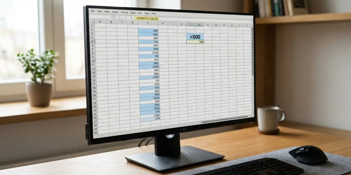
Sometimes the condition lives in the numbers themselves, such as totaling every sale above 500. Type >500 into a cell like D3, then use =SUMIF(B2:B11,D3). When the sum_range is left out, Excel adds the same cells it checks, which is exactly what is needed here. The operators >, >=, and = work the same way.
Tip: Criteria are not case sensitive, so east, East, and EAST all match the same rows.
Copy the Formula to Other Conditions
When several regions are listed down column D, lock the ranges before copying the formula down. Press F4 while each range is selected so it reads $A$2:$A$11 and $B$2:$B$11, leave the criteria reference as D2, and drag the formula down. Each row then totals its own region.
Common Problems and Fixes
The Result Is 0 Even Though Matches Exist
Check the spelling in the criteria cell and look for extra spaces before or after the word. A stray space makes East and East followed by a space two different values. Retype the criteria or clean the source cells so both match exactly.
Numbers Are Not Being Added
Numbers stored as text are skipped by SUMIF. They usually appear left-aligned or show a small green triangle in the corner. Select the cells, use the warning icon that appears, and choose Convert to Number.
The Total Looks Too Small or Too Large
The range and sum_range may be offset, such as A2:A11 paired with B3:B12. Excel then matches each condition to the wrong number. Reselect both ranges so they start on the same row and end on the same row.
A #VALUE! Error Appears
This error shows up when the formula points to another workbook that is currently closed, or when the criteria text is longer than 255 characters. Open the source workbook or shorten the criteria text.
The Formula Shows as Text Instead of a Result
If the cell displays the formula itself, the cell is probably formatted as Text. Change the format to General on the Home tab, click into the cell, and press Enter again.
Frequently Asked Questions
What is the SUMIF syntax in Excel?
The syntax is SUMIF(range, criteria, [sum_range]). The range is where Excel looks for the condition, the criteria is the rule, and the optional sum_range holds the numbers to add.
Do the range and sum_range have to be the same size?
They should be. Excel starts from the first cell of the sum_range and matches the size of the range, so mismatched or offset selections can produce totals that look wrong.
Is SUMIF case sensitive?
No. SUMIF treats upper and lower case text as the same, so east and EAST both match East.
Can SUMIF use wildcards?
Yes. An asterisk matches any number of characters and a question mark matches one character. A criteria cell containing Ea* would total every region that starts with Ea.
How can a criteria that uses greater than or less than be entered?
Put the operator and the number together in the criteria, such as >500 in a cell, and point the formula to that cell. SUMIF then adds only the values that meet the comparison.
Why do text criteria need quotation marks when typed directly into the formula?
Excel needs quotation marks to tell text apart from a cell reference or function name. Placing the criteria in a cell and referencing it avoids the issue entirely.
Can SUMIF check more than one condition at a time?
SUMIF handles one condition only. For two or more conditions, Excel offers the SUMIFS function, which uses a similar layout but starts with the sum_range.
Does SUMIF update automatically when the data changes?
Yes. As long as calculation is set to Automatic, the total refreshes whenever a matching value or a criteria cell changes.