
Learning how to use SUMIFS with multiple conditions in Excel lets a single formula total only the rows that match every rule, such as one region, one product, and one date range. The function works in Excel 2007 and later, including Microsoft 365. The steps below build the formula from scratch, then extend it with extra conditions.
Key Takeaways
- SUMIFS starts with the range to add up, followed by pairs of a criteria range and a criteria.
- A row is included only when it meets every condition, because SUMIFS applies AND logic.
- Every range in the formula must contain the same number of rows and columns.
- Placing criteria in cells keeps formulas short and avoids quotation mark mistakes.
- Up to 127 range and criteria pairs can be added to one formula.
How to Use SUMIFS with Multiple Conditions in Excel: Step-by-Step
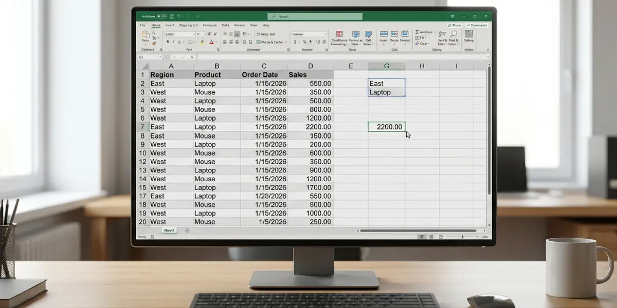
The steps use a simple sales list. Column A holds Region, column B holds Product, column C holds Order Date, and column D holds Sales. The data sits in rows 2 to 21, with headings in row 1. The goal is to total the sales for the East region and the Laptop product.
- Step 1: Check that the data is a clean block with one heading per column, no blank rows in the middle, and numbers stored as real numbers in the Sales column.
- Step 2: Type the criteria into spare cells. Enter East in cell G2 and Laptop in cell G3. Typing criteria in cells means the answer can be changed later without editing the formula.
- Step 3: Click the cell that will show the result, for example G7, and type =SUMIFS( to start the formula.
- Step 4: Add the sum range first. Type $D$2:$D$21, because SUMIFS always begins with the cells to be added up.
- Step 5: Add the first condition pair. Type $A$2:$A$21,G2, to tell Excel to look in the Region column for the value in G2.
- Step 6: Add the second condition pair. Type $B$2:$B$21,G3 to check the Product column against the value in G3.
- Step 7: Type a closing parenthesis and press Enter. The finished formula reads =SUMIFS($D$2:$D$21,$A$2:$A$21,G2,$B$2:$B$21,G3).
- Step 8: Test the result by changing G2 to West or G3 to another product. The total should update immediately.
Tip: The dollar signs lock the ranges so the formula can be copied to other cells without the ranges shifting. Press F4 right after selecting a range to add them quickly.
Add a Date or Number Condition
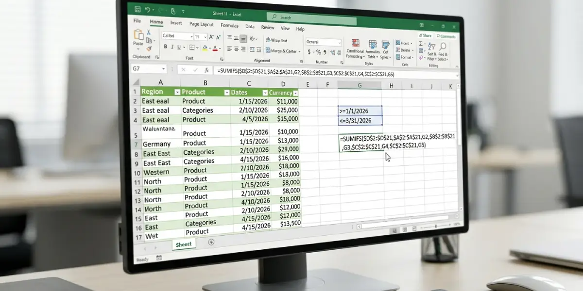
Most real reports need a third or fourth rule, and the pattern stays the same: one more criteria range, followed by one more criteria. To limit the East Laptop total to the first quarter, type >=1/1/2026 in cell G4 and <=3/31/2026 in cell G5. Then use this formula in G7:
=SUMIFS($D$2:$D$21,$A$2:$A$21,G2,$B$2:$B$21,G3,$C$2:$C$21,G4,$C$2:$C$21,G5)
The Order Date range appears twice, once for the start date and once for the end date. The same approach works for numbers. A criteria cell containing >=500 limits the total to sales of 500 or more. Dates should be entered in the format used by the computer’s regional settings.
Use Wildcards for Partial Matches
A criteria cell can contain an asterisk to match any number of characters. For instance, typing Lap* in a criteria cell matches Laptop, Laptop Stand, and any other product starting with those letters. A question mark matches exactly one character.
Tip: Criteria typed directly inside a formula must be wrapped in quotation marks, and operators combined with numbers or dates need them too. Pointing to criteria cells sidesteps that issue entirely.
Common Problems and Fixes
The Formula Returns 0 When Matching Rows Exist
This usually means the values do not match exactly. Extra spaces after a product name, or numbers stored as text, are the usual culprits. Use Trim on the source data, or select the cells and use Data, then Text to Columns, then Finish to convert text numbers to real numbers.
The Formula Returns #VALUE!
The ranges in the formula are different sizes. A sum range of D2:D21 paired with a criteria range of A2:A20 will cause this error. Make sure every range covers the same rows.
The Formula Returns #NAME?
The function name is misspelled, or a text criteria typed inside the formula is missing its quotation marks. Check the spelling of SUMIFS and switch to criteria cells to avoid the second issue.
The Total Is Too Small When Two Values Are Needed for One Column
SUMIFS requires every condition to be true at once, so a single row can never be both East and West. To total two regions, add two SUMIFS formulas together, one for each region.
The Formula Appears as Text Instead of a Result
The cell is formatted as Text. Change the format to General on the Home tab, click into the cell, and press Enter again.
The Sum Range Was Placed After the Criteria
Users familiar with SUMIF often put the sum range last. In SUMIFS the sum range comes first, so the formula must start with the cells to be added up.
Frequently Asked Questions
How many conditions can SUMIFS handle in Excel?
SUMIFS accepts up to 127 pairs of criteria range and criteria in a single formula. Most everyday reports need only two to four.
Does SUMIFS use AND or OR logic with multiple conditions?
SUMIFS uses AND logic, so a row is added only when it meets every condition. For OR logic, add together separate SUMIFS formulas, one for each alternative.
What is the correct order of arguments in SUMIFS?
The first argument is the sum range, followed by the first criteria range, the first criteria, and then any further criteria range and criteria pairs.
Can SUMIFS use criteria stored in other cells?
Yes. Entering a cell reference as the criteria makes Excel use that cell’s value. This keeps the formula short and lets the answer change when the cell is edited.
How can SUMIFS sum values between two dates?
Use the date column as a criteria range twice. One criteria is a greater than or equal to the start date, and the other is a less than or equal to the end date.
Do the ranges in SUMIFS need to be the same size?
Yes. The sum range and every criteria range must have the same number of rows and columns, or the formula returns a #VALUE! error.
Can SUMIFS match partial text?
Yes. Wildcards work in the criteria. An asterisk matches any number of characters, and a question mark matches a single character.
Why does SUMIFS return 0 even though matching data exists?
The most common causes are hidden extra spaces in the data, numbers stored as text, or criteria that do not match the cell values exactly. Cleaning the source data usually fixes it.
Is SUMIFS case sensitive?
No. SUMIFS treats East, east, and EAST as the same value when matching text criteria.