
Using VLOOKUP with an exact match in Excel is the most reliable way to pull the correct value from a table, since it stops the formula from guessing at close matches. This guide walks through the exact formula setup, step by step, so lookups return the right result every time.
Key Takeaways
- Setting the fourth argument in VLOOKUP to FALSE or 0 forces an exact match.
- The lookup column must be sorted correctly for approximate matches, but exact match works regardless of sort order.
- The lookup value must match the data type and formatting in the table exactly, including text versus numbers.
- The #N/A error almost always means the lookup value was not found exactly as typed.
- Absolute references keep the table range fixed when the formula is copied down a column.
Step-by-Step Guide to VLOOKUP with an Exact Match
- Step 1: Click the cell where the result should appear.
- Step 2: Type =VLOOKUP( to begin the formula.
- Step 3: Enter the lookup value first. This can be a direct reference to a cell, such as A2, or a value typed in quotes.
- Step 4: Add a comma, then select the full range of the table being searched, including the column with the lookup values and every column to its right that contains data to retrieve.
- Step 5: Add another comma, then type the column number within that selected range that holds the value to return. Counting starts at 1 from the leftmost column of the selected range, not from the worksheet’s column letters.
- Step 6: Add a final comma, then type FALSE or 0 to force an exact match rather than an approximate one.
- Step 7: Close the parenthesis and press Enter to run the formula.

Tip: Press F4 right after selecting the table range to lock it with dollar signs, like $A$2:$D$100. This keeps the range fixed when the formula gets copied to other rows, which is where most VLOOKUP formulas fall apart.
Example Formula
A formula pulling a price from column D of a table in A2:D500, based on a product code in A2, looks like this: =VLOOKUP(A2,$A$2:$D$500,4,FALSE). Every part of that formula matters: the lookup value, the locked range, the column number, and the FALSE at the end that forces the exact match.
Copying the Formula Down a Column
Once the first VLOOKUP formula returns the correct result, copying it down a full column is usually the next step, and this is where an unlocked range becomes a problem.
- Step 1: Confirm the table range in the formula uses dollar signs, such as $A$2:$D$500.
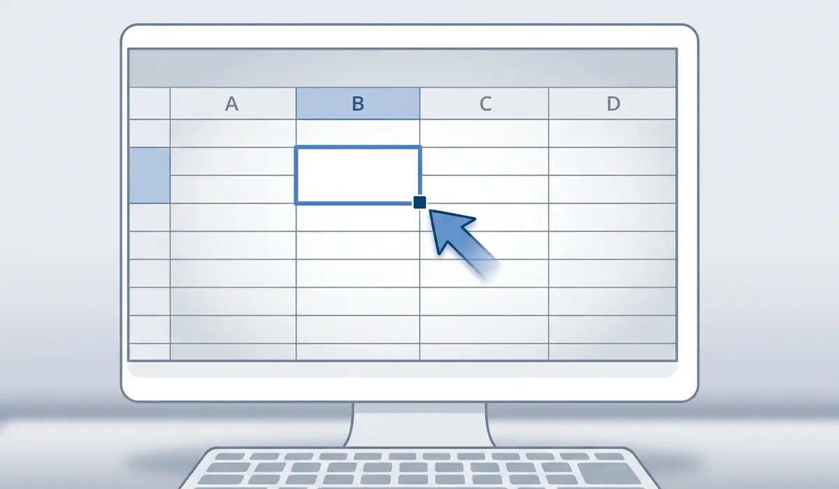
- Step 2: Click the small square at the bottom-right corner of the cell containing the formula.
- Step 3: Drag it down through every row that needs the lookup, or double-click the square to fill automatically to the end of an adjacent data column.
- Step 4: Spot-check a few rows in the middle and at the bottom of the range to confirm the results are pulling from the correct table.

Common Problems and Fixes
- The formula returns #N/A even though the value clearly exists in the table – trailing spaces or inconsistent formatting between the lookup value and the table entry are the usual cause. Use TRIM on both values to strip extra spaces and try again.
- The formula returns #N/A because one cell holds text and the other holds a number – a product code stored as text in one cell and as a number in another will never match exactly. Convert both to the same data type before running the lookup.
- The formula returns the wrong value from a different row – this usually means the fourth argument was left blank or set to TRUE, which allows an approximate match. Setting it to FALSE or 0 fixes this immediately.
- The range shifts or shrinks after copying the formula down – the table range was not locked with dollar signs before copying. Add $ symbols to the range and copy the formula again.
- The wrong column number returns an unrelated value – remember that column numbering starts at 1 from the first column selected in the range, not from the worksheet’s actual column letter.
Frequently Asked Questions
What does FALSE mean in a VLOOKUP formula?
FALSE in the fourth argument tells VLOOKUP to return a result only when it finds a value that matches the lookup value exactly, rather than the closest approximate match.
Can 0 be used instead of FALSE for an exact match?
Yes. Excel treats 0 and FALSE as equivalent in the fourth argument of VLOOKUP, and both force an exact match.
Why does VLOOKUP return #N/A when the value is clearly in the table?
This typically happens due to extra spaces, mismatched data types between text and numbers, or a lookup value that does not match the table entry exactly, including capitalization or hidden formatting differences.
Does the lookup column need to be sorted for an exact match?
No. Sorting only matters for approximate match lookups. Exact match VLOOKUP works correctly regardless of how the data is ordered.
Can VLOOKUP look to the left of the lookup column?
No. VLOOKUP only searches to the right of the column containing the lookup value within the selected range, so the return column must sit to the right of it.
What happens if the fourth argument is left out entirely?
Excel defaults to TRUE, which performs an approximate match. Leaving it out is one of the most common reasons a lookup returns an incorrect result.
How does column numbering work inside the VLOOKUP formula?
Numbering starts at 1 for the first column of the selected range, not the worksheet’s column letter, so the return column number depends entirely on where the range selection begins.
Can VLOOKUP match text that has different capitalization?
Yes. VLOOKUP is not case-sensitive, so ‘apple’ and ‘APPLE’ are treated as an exact match.
How can an exact match formula be locked so it does not shift when copied?
Adding dollar signs to the table range, such as $A$2:$D$500, locks it in place so the range stays fixed no matter where the formula is copied.