
A two-way lookup with INDEX and MATCH in Excel returns the value that sits where one chosen row and one chosen column cross. Think of it like finding a seat in a theater: one clue gives the row, another gives the seat number, and together they point to exactly one spot. This guide builds the formula from scratch using a simple sales table.
Key Takeaways
- One MATCH finds the row number, a second MATCH finds the column number, and INDEX returns the cell where they meet.
- The formula pattern is =INDEX(data, MATCH(row item, row labels, 0), MATCH(column item, column headers, 0)).
- Always use 0 as the last MATCH argument so Excel looks for an exact match.
- The data range and both label ranges must line up in size and position.
Step-by-Step Guide to Build a Two-Way Lookup with INDEX and MATCH in Excel
The steps below use a sample table. Region names are in A2:A5, month names are in B1:E1, and the sales figures are in B2:E5. The lookup inputs go in G1 and G2, and the result goes in G3. Adjust the references to fit the real worksheet.
Set Up the Lookup Cells
- Step 1: Confirm the table has row labels down the left side (A2:A5) and column headers across the top (B1:E1), with the values in B2:E5.
- Step 2: In cell G1, type the row item to look up, for example South.
- Step 3: In cell G2, type the column item to look up, for example Mar.
- Step 4: Click cell G3, which will hold the result.
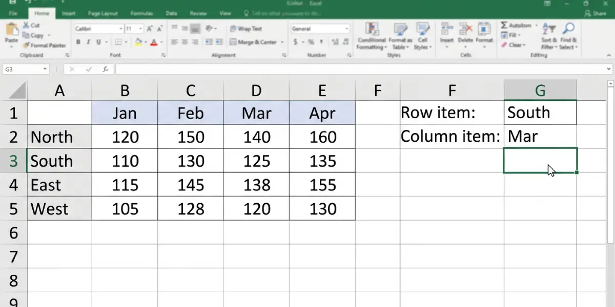
Tip: Keeping the lookup inputs in their own cells, rather than typing the names inside the formula, makes the lookup reusable. Changing G1 or G2 updates the answer instantly.
Build the Formula in Pieces
- Step 5: Find the row position by typing =MATCH(G1,A2:A5,0) in any spare cell. With South in G1, the result is 2, because South is the second item in the list.
- Step 6: Find the column position by typing =MATCH(G2,B1:E1,0) in another spare cell. With Mar in G2, the result is 3, because Mar is the third header.
- Step 7: Combine both into INDEX by typing this in G3: =INDEX(B2:E5,MATCH(G1,A2:A5,0),MATCH(G2,B1:E1,0))
- Step 8: Press Enter. Excel returns the value from the second row and third column of B2:E5, which is the South figure for March.
- Step 9: Delete the two spare test cells from Steps 5 and 6, since the final formula no longer needs them.
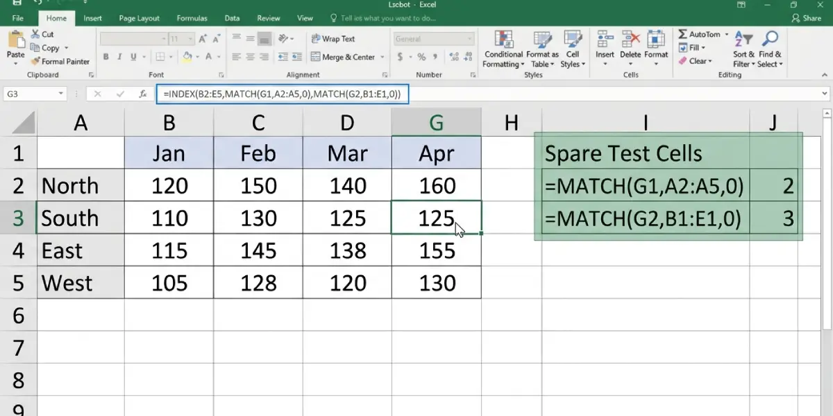
The key is to read the formula from the inside out. Each MATCH answers a position question, and INDEX uses those two positions as coordinates inside B2:E5.
Test the Result
- Step 10: Change G1 to a different region and G2 to a different month, then check the result against the table by eye.
- Step 11: Optionally, select G1 and G2 and use Data, then Data Validation, then List to create dropdowns that pull from A2:A5 and B1:E1. This prevents typos in the lookup inputs.
Tip: Press F4 while the cursor is inside each range reference to lock it, turning B2:E5 into $B$2:$E$5. Locked references stay put when the formula is copied to other cells.
Common Problems and Fixes
The Formula Returns #N/A
This means one of the MATCH functions could not find its item. Check the spelling of the entry in G1 or G2, and look for stray spaces before or after the text. A header that looks like Mar may actually be stored as March or contain a trailing space. Retyping the entry or cleaning the label with the TRIM function usually clears it.
Numbers or Dates Do Not Match
If the headers are numbers or dates, the lookup entry must be the same type. A number stored as text will not match a true number, even though both look identical. Convert the text to numbers, or retype the value so both sides are the same type.
The Formula Returns the Wrong Value
The most common cause is a missing third argument in MATCH. Without 0, Excel defaults to an approximate match and can land on the wrong position. Make sure both MATCH functions end with ,0).
The Formula Returns #REF!
This happens when a MATCH result points outside the INDEX range. It is usually caused by a data range that does not line up with the label ranges. If the labels run from A2 to A5, the data range must also start at row 2 and end at row 5. The same rule applies to columns.
The Result Is Zero When a Cell Looks Empty
When the matching cell in the table is blank, INDEX returns 0. Fill the blank cell with the intended value, or accept the zero as the result for an empty cell.
Frequently Asked Questions
What does a two-way lookup with INDEX and MATCH do in Excel?
It returns the value found at the intersection of a specific row and a specific column in a table. One MATCH locates the row, another MATCH locates the column, and INDEX retrieves the value at that position.
Why is 0 used as the last argument in MATCH?
The 0 tells MATCH to find an exact match. Leaving it out can cause Excel to return an approximate position, which gives incorrect results with unsorted labels.
Does the data range need to include the row and column labels?
No. The INDEX range should contain only the values, such as B2:E5. The row labels and column headers are referenced separately inside the two MATCH functions.
Can the lookup inputs be typed straight into the formula?
Yes, text entries can be typed inside the formula in place of cell references. Using cells such as G1 and G2 is easier to change and less error-prone.
Why does the formula return #N/A?
One of the MATCH functions cannot find its lookup item in the label range. Typos, extra spaces, and mismatched data types, such as a number stored as text, are the usual causes.
Is the lookup case sensitive?
No. MATCH ignores uppercase and lowercase, so south and South return the same position.
Do the row and column labels have to be sorted?
No. With 0 as the match type, the labels can be in any order.
Can the formula be copied to other cells?
Yes. Lock the ranges with absolute references such as $B$2:$E$5 so they do not shift when the formula is copied, and point each copy at its own lookup input cells.