
Learning how to add sparklines to an Excel worksheet takes about a minute, and the payoff is immediate: a tiny chart sits right inside a cell, showing the trend of a whole row of numbers at a glance. This works best when the data is laid out in rows or columns with one series per line, such as monthly sales per product. The steps below cover the full process, from selecting the data to styling the result.
Key Takeaways
- Sparklines are inserted from the Insert tab, in the Sparklines group, by choosing Line, Column, or Win/Loss.
- The Data Range holds the numbers, and the Location Range is the cell (or cells) where the mini chart appears.
- Dragging the fill handle copies a sparkline down a column or across a row.
- The Sparkline tab lets you highlight high and low points, change colors, and handle hidden or empty cells.
How to Add Sparklines to an Excel Worksheet Step by Step
The example here assumes product names in column A, monthly figures in B2:G2 through B6:G6, and an empty column H waiting for the sparklines.
- Step 1: Open the workbook and make sure the numbers sit in a clean range. Each row (or column) should hold one data series, with no merged cells in the middle.
- Step 2: Click the first empty cell where the sparkline should appear, such as H2. Leaving a blank column next to the data keeps things tidy.
- Step 3: Go to the Insert tab on the ribbon and find the Sparklines group.
- Step 4: Choose the type: Line for trends over time, Column for comparing values, or Win/Loss for positive and negative outcomes.
- Step 5: In the Create Sparklines dialog box, click the Data Range box and select the numbers for that row, for example B2:G2.
- Step 6: Check the Location Range box. It should show the cell chosen in Step 2, such as $H$2.
- Step 7: Click OK. The mini chart appears inside the cell.
- Step 8: Drag the fill handle (the small square at the bottom-right corner of the cell) down to H6 to create sparklines for the remaining rows.
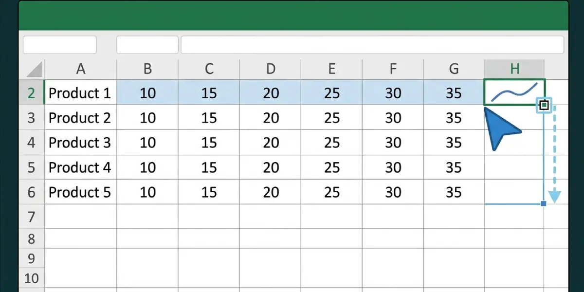
Tip: To create every sparkline in one go, select the whole location range first (H2:H6), then choose the sparkline type and set the Data Range to B2:G6. Excel matches each row of data to its own cell automatically.
Choosing the Right Sparkline Type
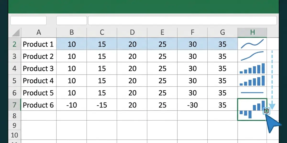
Line sparklines suit data that moves over time, like weekly website visits. Column sparklines make it easy to compare individual values side by side. Win/Loss sparklines ignore the size of the numbers and only show whether each value is positive or negative, which fits profit and loss or pass and fail results.
Customize Sparklines After Adding Them
A sparkline on its own is useful, but a few adjustments make it easier to read. Click any cell that contains a sparkline and a Sparkline tab appears on the ribbon with all the formatting options.
Highlight Key Points
In the Show group, tick High Point, Low Point, Negative Points, First Point, Last Point, or Markers (Markers is available for line sparklines). Ticking High Point and Low Point is a popular choice because the peak and dip stand out instantly.
Change the Style and Color
Use the Style gallery for a ready-made look, or open Sparkline Color and Marker Color to pick custom colors. A darker line with a single bright marker for the last point is an easy way to draw the eye to the latest value.
Make the Sparkline Bigger
Sparklines fill the cell they live in, so widening the column or increasing the row height makes the chart larger and easier to read.
Tip: When sparklines in a column are meant to be compared with each other, open Axis in the Group section and set the vertical axis minimum and maximum to Same for All Sparklines. Otherwise, each sparkline scales itself to its own data, and a small series can look as dramatic as a large one.
Common Problems and Fixes
The Location Reference Is Not Valid
This warning appears when the shape of the Location Range does not match the Data Range. If the data covers five rows, the location needs five cells. Re-open the dialog box and correct either range, or insert sparklines one row at a time.
The Sparkline Looks Empty or Flat
Numbers stored as text will not plot. Convert them to real numbers, then check that the Data Range actually covers the values and not a label column. A flat line can also mean every value in the row is the same.
Data in Hidden Rows or Columns Is Missing
By default, sparklines ignore hidden cells. Select the sparkline, open Edit Data on the Sparkline tab, choose Hidden and Empty Cells, and tick Show data in hidden rows and columns.
Gaps Appear Where Cells Are Empty
In the same Hidden and Empty Cells dialog box, set empty cells to show as Gaps, Zero, or Connect data points with line, depending on how the missing values should be treated.
The Sparkline Will Not Delete
Pressing the Delete key on a cell does not remove its sparkline. Select the cell, go to the Sparkline tab, and click Clear. To remove a whole group at once, use the arrow next to Clear and choose Clear Selected Sparkline Groups.
Frequently Asked Questions
Where do I find the sparkline option in Excel?
Sparklines are on the Insert tab of the ribbon, in the Sparklines group. The three choices there are Line, Column, and Win/Loss.
Can I add sparklines to more than one row at once?
Yes. Select the full location range, such as H2:H6, then choose a sparkline type and set the Data Range to cover all the matching rows. Excel creates one sparkline per row.
How do I copy a sparkline to other cells?
Select the cell with the sparkline and drag the fill handle across or down. The new sparklines join the same group and share its formatting.
How do I change a sparkline from line to column?
Click a cell containing the sparkline, open the Sparkline tab, and choose Line, Column, or Win/Loss in the Type group. The change applies to the whole group.
How do I show the highest and lowest values on a sparkline?
Select the sparkline, go to the Sparkline tab, and tick High Point and Low Point in the Show group. Each point is marked with a contrasting color.
Can I type text in a cell that has a sparkline?
Yes. A sparkline sits in the background of the cell, so typed text or a number appears over it. Many people use this to show a value next to its trend, and a larger row height keeps both readable.
How do I change the data a sparkline uses?
Select the sparkline, open the Sparkline tab, click Edit Data, and choose Edit Group Location and Data or Edit Single Sparkline’s Data. Then pick the new range.
How do I remove sparklines from a worksheet?
Select the cell or cells, open the Sparkline tab, and click Clear. The Delete key does not remove them.