
Need to replace VLOOKUP with INDEX and MATCH in Excel? The conversion takes less than a minute once the four parts of the old formula are mapped to the new one. The example below uses a product list, but the same pattern works for any lookup table.
Key Takeaways
- VLOOKUP’s column number is replaced by a full return column that INDEX reads from.
- MATCH finds the row of the lookup value inside a single lookup column.
- The pattern is =INDEX(return column, MATCH(lookup value, lookup column, 0)).
- Locking the ranges with absolute references keeps the formula accurate when filled down.
- The finished formula keeps working if columns are inserted or deleted in the table.
How to Replace VLOOKUP with INDEX and MATCH in Excel Step by Step
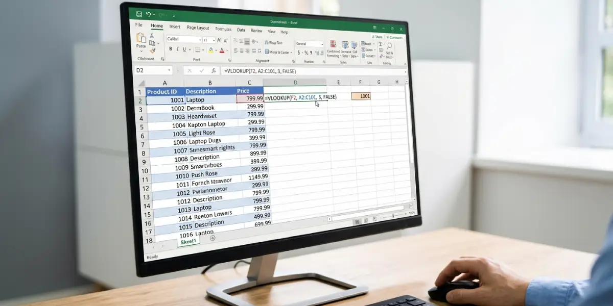
The example data sits in A2:C101. Column A holds Product ID, column B holds Product Name, and column C holds Price. The lookup value is typed in cell F2, and the result appears in G2. The existing formula in G2 is =VLOOKUP(F2,A2:C101,3,FALSE).
Convert the Formula
- Step 1: Click the cell that holds the VLOOKUP formula and read its four parts. In the example, F2 is the lookup value, A2:C101 is the table, 3 is the column number, and FALSE means exact match.
- Step 2: Find the return column. The 3 in the old formula points to the third column of the table, which is column C. The return range becomes C2:C101.
- Step 3: Find the lookup column. VLOOKUP always searches the first column of the table, so the lookup range is A2:A101.
- Step 4: Build the MATCH part by typing =MATCH(F2,A2:A101,0) in a spare cell. The 0 forces an exact match, the same job FALSE did in VLOOKUP. The cell returns a row position, such as 14.
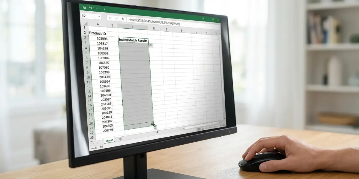
- Step 5: Wrap that MATCH inside INDEX. In G2, type =INDEX(C2:C101,MATCH(F2,A2:A101,0)) and press Enter. INDEX takes the row number from MATCH and returns the value from that row of column C.
- Step 6: Compare the new result with the old VLOOKUP result for the same lookup value. Both should show the same price.
Tip: Think of MATCH as a person reading down a list to say ‘it’s the 14th name’, and INDEX as the person who walks to the 14th row of another list and reads out what is written there. Each does one small job, and together they replace the single VLOOKUP.
Apply the New Formula to Every Row
- Step 7: Lock the ranges so they do not shift when the formula is copied down. Click inside the formula, select each range, and press F4 to add dollar signs. The result is =INDEX($C$2:$C$101,MATCH(F2,$A$2:$A$101,0)). On some laptops, Fn+F4 is needed. Leave F2 unlocked so it moves to F3, F4, and so on.
- Step 8: Double-click the fill handle, the small square in the bottom-right corner of the selected cell, to copy the formula down the column as far as the data in the neighboring column extends.
- Step 9: Spot-check a few rows, then clear or overwrite the old VLOOKUP formulas.
Tip: To look up a value to the left of the lookup column, only the two ranges change. For example, to find a Product ID from a Product Name, use =INDEX(A2:A101,MATCH(F2,B2:B101,0)). VLOOKUP cannot do this, but the INDEX and MATCH pattern handles it with no extra steps.
Common Problems and Fixes
The Formula Returns #N/A
This means MATCH could not find the lookup value. Check for extra spaces at the start or end of the value, and confirm that both the lookup value and the lookup column contain the same kind of data. If the problem is a typo or a missing item, correct the source value. If blanks are expected, wrap the whole formula in IFERROR and give it a fallback such as 0 or an empty text value.
Numbers Look Identical but Still Fail to Match
One side is probably stored as text and the other as a number. A green triangle in the corner of a cell is a common clue. Convert the text entries to numbers, or retype the lookup value so both sides share one format.
The Result Is the Wrong Row
The last argument of MATCH was probably left out or set to 1. Without the 0, MATCH looks for an approximate match and expects sorted data. Always end the MATCH with ,0 for an exact match.
The Result Is Off by One or More Rows
INDEX and MATCH ranges must start on the same row. If the return range is C3:C101 while the lookup range is A2:A101, every result slides down one row. Make both ranges begin and end on the same rows.
The Results Change After Filling the Formula Down
The ranges were not locked. Press F4 inside each range reference to add dollar signs, then copy the formula down again.
The Formula Shows #REF!
A column or row used by the formula was deleted. Rebuild the broken reference by selecting the correct range inside the formula.
Frequently Asked Questions
What is the basic formula to replace VLOOKUP with INDEX and MATCH?
The pattern is =INDEX(return column, MATCH(lookup value, lookup column, 0)). The return column holds the answer, the lookup column holds the value being searched for, and the 0 requests an exact match.
What does the 0 in the MATCH function mean?
The 0 sets the match type to exact match. It works like FALSE in VLOOKUP and tells Excel to return a result only when the value is found exactly.
Where does the VLOOKUP column number go in INDEX and MATCH?
The column number is no longer typed. Instead, the actual return column, such as C2:C101, is placed in the first argument of INDEX. The column is selected directly, so inserting a new column does not break the result.
Can INDEX and MATCH look up a value to the left?
Yes. Because the lookup column and the return column are separate ranges, the return column can sit on either side. Swap the two ranges to look left.
Do the INDEX and MATCH ranges have to be the same size?
Yes, they should start and end on the same rows. If the sizes or starting rows differ, MATCH returns a position that points to the wrong row of the return column.
How do I replace an approximate match VLOOKUP with INDEX and MATCH?
VLOOKUP with TRUE or no fourth argument uses an approximate match. For INDEX and MATCH, set the last argument of MATCH to 1 instead of 0, and keep the lookup column sorted in ascending order.
How can the #N/A error be hidden when no match exists?
Wrap the formula in IFERROR, with the INDEX and MATCH formula as the first argument and a fallback value as the second. The fallback can be 0 or an empty text value.
Does the new formula work in all versions of Excel?
Yes. INDEX and MATCH have been part of Excel for many years and work in desktop Excel for Windows and Mac, as well as Excel for the web.
Why use F4 when filling the formula down?
F4 turns relative references into absolute ones by adding dollar signs. This keeps the lookup and return ranges fixed while only the lookup value changes from row to row.