
Tired of resizing chart ranges every time a new row of data arrives? Excel Charts: build a dynamic chart with named ranges is the fix, because the chart reads its data from formulas that grow and shrink on their own. The whole setup takes about ten minutes, and it works in every modern version of Excel for Windows and Mac.
Key Takeaways
- A dynamic chart pulls its data from named ranges built with the OFFSET and COUNTA functions.
- Each named range must include the workbook name or sheet name when it is entered into the chart series.
- Once connected, the chart expands automatically when rows are added at the bottom of the data.
- The data must sit in a continuous column with no blank cells in between.
Step-by-Step Guide to Build a Dynamic Chart with Named Ranges
The example below assumes a simple monthly sales table on a sheet named Sheet1. Months are in column A and sales figures are in column B, with headers in row 1 and data starting in row 2. Adjust the cell references to match your own layout.
Create the Named Ranges
- Step 1: Open the workbook and confirm the data is in a continuous block with a header in A1 and B1 and no empty rows inside the data.
- Step 2: Go to the Formulas tab and select Name Manager, then click New.
- Step 3: In the Name box, type ChartMonths. Leave the Scope set to Workbook.
- Step 4: In the Refers to box, delete the existing content and enter this formula: =OFFSET(Sheet1!$A$2,0,0,COUNTA(Sheet1!$A:$A)-1,1). Click OK.
- Step 5: Click New again. In the Name box, type ChartSales.
- Step 6: In the Refers to box, enter: =OFFSET(Sheet1!$B$2,0,0,COUNTA(Sheet1!$B:$B)-1,1). Click OK, then close Name Manager.
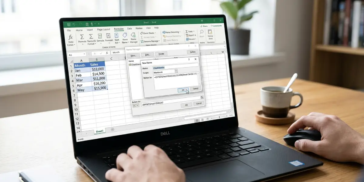
Here is what the formula does. OFFSET starts at the first data cell, then COUNTA counts how many filled cells exist in the column. Subtracting 1 removes the header from the count, so the range always covers exactly the data rows. Think of it as a rubber band that stretches to fit whatever is inside.
Tip: Keep nothing else in columns A and B below or above the table, such as notes or totals, because COUNTA counts every non-empty cell in the full column.
Build the Chart and Connect the Names
- Step 7: Select any cell in the data table, go to the Insert tab, and choose a chart such as Clustered Column or Line. Excel creates a standard chart based on the current cells.
- Step 8: Right-click the chart and choose Select Data.
- Step 9: Under Legend Entries (Series), select the sales series and click Edit.
- Step 10: In the Series values box, replace the cell range with the named range in this format: =Book1.xlsx!ChartSales. Replace Book1.xlsx with the exact file name of the workbook, including the extension. Click OK.
- Step 11: Under Horizontal (Category) Axis Labels, click Edit. In the Axis label range box, enter =Book1.xlsx!ChartMonths using the same workbook name, then click OK twice.
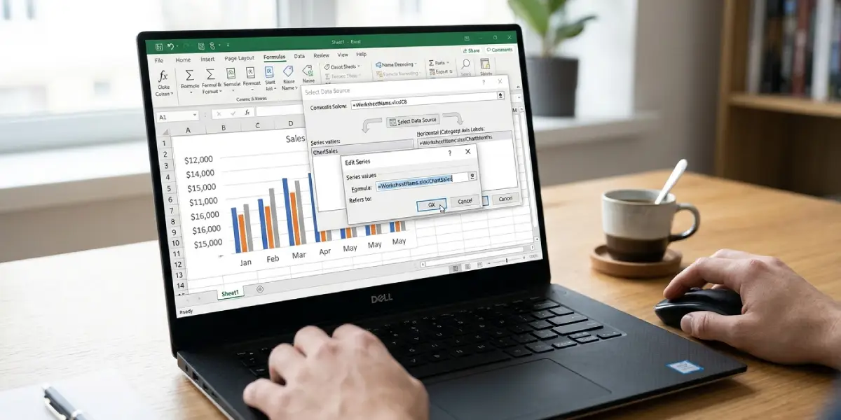
Excel may rewrite the reference to include the sheet name or the workbook name once the entry is accepted. That is normal and means the connection worked.
Test the Dynamic Behavior
- Step 12: Type a new month in the first empty cell of column A and a value in the matching cell of column B.
- Step 13: Watch the chart. The new data point should appear immediately without any change to the series settings.
Tip: Save the workbook before building the series references. A file name that has never been saved can cause the named range entry to fail or point to the wrong workbook.
Common Problems and Fixes
The Reference Is Not Valid Error Appears
This message usually means the workbook name is typed incorrectly or the named range does not exist. Open Name Manager and confirm the exact spelling of ChartMonths and ChartSales. Then check that the workbook name in the series formula matches the file name exactly, including the extension. If the file name contains spaces, wrap it in single quotes, such as =’Sales Report.xlsx’!ChartSales.
The Chart Shows Extra Blank Points
Extra empty points mean COUNTA is counting cells that should not be included. Check the column for stray notes, totals, or a second table beneath the data and remove them, or move them to another column.
The Chart Does Not Update When New Rows Are Added
Confirm that the series values box shows a named range and not regular cell addresses. If Excel converted the name back into a fixed range, repeat the Select Data steps and re-enter the named range.
The Chart Is Missing the Last Row of Data
This happens when the header row is not counted as expected. If the table has no header in row 1, remove the minus 1 from the COUNTA part of the formula. If there are two header rows, subtract 2 instead.
The Series Breaks After Renaming the File
The series formula stores the workbook name. After renaming or saving a copy under a new name, open Select Data and update the workbook name in both series entries.
Frequently Asked Questions
Can a dynamic chart with named ranges work with more than one data series?
Yes. Create one named range for each series of values, using the same OFFSET and COUNTA pattern, then add each name as its own series through Select Data.
Do named ranges work for charts on a different sheet than the data?
Yes. Named ranges set to Workbook scope can be used by a chart on any sheet. The formulas inside the names must still reference the sheet that holds the data.
Why must the workbook name be typed in the series formula?
Excel requires a named range in a chart series to be qualified with the workbook or sheet name. Without it, the entry is rejected as an invalid reference.
Is an Excel Table a simpler option than named ranges?
An Excel Table also expands charts automatically, but named ranges give more control, such as showing only the latest 12 data points. For the task of building a dynamic chart with named ranges, the OFFSET method shown here is the right approach.
How can the chart show only the last 12 entries?
Change the OFFSET formula so the starting row moves down as data grows. For values, use =OFFSET(Sheet1!$B$1,COUNTA(Sheet1!$B:$B)-12,0,12,1), and use the same pattern for the category names in column A.
What happens if there are blank cells inside the data?
COUNTA only counts filled cells, so a gap shifts the count and the chart will cut off the last entries. Fill the gap or remove the empty row before relying on the chart.
Does this method work in Excel for Mac?
Yes. The Name Manager is on the Formulas tab, and the Select Data dialog works the same way, so the steps are identical.
Will the named ranges survive if the workbook is shared with someone else?
Yes, as long as the file is shared as a workbook. The names and the chart connections are stored inside the file, so the chart keeps updating on the other person’s computer.
Can the dynamic chart be edited later if the data columns change?
Yes. Open Name Manager, select the name, and edit the formula in the Refers to box. The chart picks up the change right away.