
Need to pull one exact number out of a PivotTable and drop it into a report? Learning to use GETPIVOTDATA in Excel makes that possible, because the formula finds a value by its field names instead of by its cell position. That means the number stays correct even when the PivotTable is rearranged, filtered, or refreshed.
Key Takeaways
- GETPIVOTDATA returns a value from a PivotTable based on field names and items, not on cell addresses.
- The easiest way to create the formula is to type an equals sign in a cell outside the PivotTable and click the value needed.
- Typed text in the formula can be swapped for cell references to make the result dynamic.
- Most errors come from a hidden item, a misspelled field name, or a PivotTable cell reference that no longer points to the PivotTable.
How to Use GETPIVOTDATA in Excel Step by Step
The steps below assume a PivotTable that shows Region in the Rows area and Sum of Sales in the Values area, starting in cell A3. The same logic applies to any PivotTable.
Create a GETPIVOTDATA Formula by Clicking
- Step 1: Confirm that the PivotTable is built and that the item needed is visible in it. For example, the row for the East region must appear in the PivotTable.
- Step 2: Click an empty cell outside the PivotTable, such as H6, where the result should appear.
- Step 3: Type an equals sign (=) to start the formula.
- Step 4: Click the PivotTable cell that holds the value needed, such as the Sum of Sales figure on the East row.
- Step 5: Press Enter. Excel writes the full GETPIVOTDATA formula automatically, with the data field name and the Region item filled in.
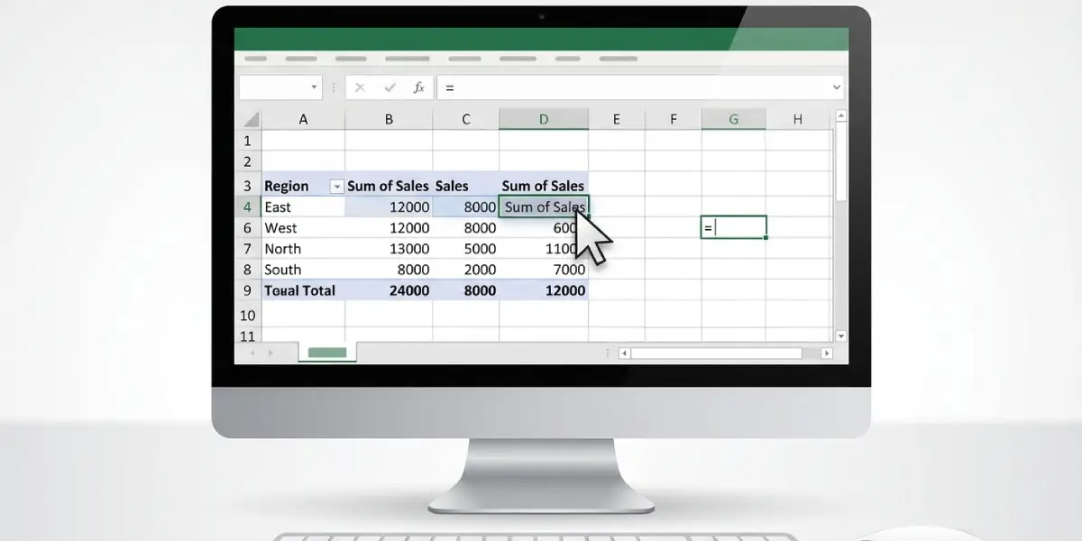
Tip: Clicking a cell is far safer than typing the formula by hand, because Excel copies the field names and items exactly as the PivotTable stores them.
Read the Formula Before Changing It
The syntax is GETPIVOTDATA(data_field, pivot_table, [field1, item1], [field2, item2], and so on). Each part has a simple job:
- data_field is the name of the value column, such as Sum of Sales, entered as text.
- pivot_table is any cell inside the PivotTable, usually the top-left cell, such as $A$3.
- Each field and item pair narrows the result, for example the field Region paired with the item East.
Think of it like a street address: the data field is the city, the PivotTable reference is the neighborhood, and each field and item pair is a more specific turn until the exact house is found.
Replace Typed Text With Cell References
Auto-generated formulas contain fixed text, so changing the region means editing the formula. Cell references remove that chore.
- Step 1: Type the text Sum of Sales in cell H1, the text Region in cell H2, and the region name East in cell H3. Each entry must match the PivotTable exactly.
- Step 2: In cell H6, enter the formula =GETPIVOTDATA(H1,$A$3,H2,H3).
- Step 3: Press Enter. The result matches the East row of the PivotTable.
- Step 4: Change the entry in H3 to West or North, and the formula returns the matching value instantly.
Return the Grand Total
- Step 1: Click the cell where the grand total should appear.
- Step 2: Enter =GETPIVOTDATA(H1,$A$3), where H1 holds the data field name and A3 sits inside the PivotTable.
- Step 3: Press Enter. With no field and item pairs, the formula returns the grand total for that data field.
Tip: Make sure the Grand Totals setting is turned on for the PivotTable. If grand totals are hidden, this formula has nothing to return.
Turn Automatic GETPIVOTDATA On or Off
Excel inserts GETPIVOTDATA by default whenever a PivotTable cell is clicked during formula entry. Some people prefer a normal cell reference such as =B5 instead. The setting is easy to change.
- Step 1: Click any cell inside the PivotTable.
- Step 2: Open the PivotTable Analyze tab on the ribbon.
- Step 3: In the PivotTable group, click the arrow beside Options.
- Step 4: Click Generate GetPivotData to clear the check mark and turn the feature off, or click it again to turn it back on.
Common Problems and Fixes
The Formula Returns #REF!
This is the most frequent error. It appears when the item requested is not visible in the PivotTable, for example when a filter or slicer hides the East region. Clear the filter so the item shows again, and the value returns. The error also appears when a field name or item is misspelled, or when the data field name does not match the PivotTable.
The Data Field Name Does Not Match
The data field must match the name shown in the PivotTable header, such as Sum of Sales. If that header was renamed to something like Total Sales, the renamed text must be used instead. Copying the header text into a cell and referencing it avoids typing mistakes.
The Pivot Table Reference Is Wrong
The second argument must point to a cell inside the PivotTable. If the PivotTable was moved or deleted, the reference may land on an empty cell and the formula fails. Update the reference to a cell in the current PivotTable.
The Formula Shows a Plain Cell Reference Instead
If clicking a PivotTable cell creates a reference like =B5, Generate GetPivotData is turned off. Turn it back on from the PivotTable Analyze tab using the steps above, then create the formula again.
The Result Does Not Update After the Source Data Changes
The PivotTable itself must be refreshed before GETPIVOTDATA shows new numbers. Click inside the PivotTable, then choose Refresh on the PivotTable Analyze tab, or press Alt+F5.
A Date Item Returns an Error
Dates must be supplied as real dates, not as loose text. Use a cell that contains a true date value as the item, and make sure that exact date appears in the PivotTable. If the dates are grouped by month or year, the item must match the grouped label instead.
Frequently Asked Questions
What does GETPIVOTDATA do in Excel?
GETPIVOTDATA retrieves a specific value from a PivotTable by using field names and items. The result stays tied to the data itself, so it holds up when the PivotTable layout changes.
Why does Excel insert GETPIVOTDATA automatically when a PivotTable cell is clicked?
Excel has a setting called Generate GetPivotData that is turned on by default. It creates the formula whenever a PivotTable cell is clicked while a formula is being entered.
How can automatic GETPIVOTDATA be turned off?
Click a cell in the PivotTable, open the PivotTable Analyze tab, click the arrow beside Options in the PivotTable group, and clear the Generate GetPivotData check mark.
What is the syntax of GETPIVOTDATA?
The syntax is GETPIVOTDATA(data_field, pivot_table, [field1, item1], [field2, item2], and so on). The data field is the value name, the pivot table is a cell inside the PivotTable, and the optional pairs narrow the result.
Why does GETPIVOTDATA return #REF!?
The item is usually hidden by a filter or slicer, a field name or item is misspelled, or the data field name does not match the PivotTable. Fix the item visibility or correct the names, and the value returns.
Can GETPIVOTDATA return the grand total of a PivotTable?
Yes. Enter only the data field and a cell inside the PivotTable, such as =GETPIVOTDATA(H1,$A$3), and the formula returns the grand total for that data field.
Can cell references be used inside GETPIVOTDATA?
Yes. The data field, the field names, and the items can all come from cells. This lets one formula return different results when the contents of those cells change.
Does GETPIVOTDATA update when the PivotTable is refreshed?
Yes. After the PivotTable is refreshed, the formula reflects the updated numbers. The PivotTable must be refreshed first, because the formula reads from the PivotTable and not from the source data directly.
Can GETPIVOTDATA read a PivotTable on another worksheet?
Yes. Reference a cell in the PivotTable with the sheet name included, such as Sheet1!$A$3, and the formula reads from that PivotTable.