
Knowing how to apply a color scale in Excel turns a wall of numbers into a heat map that the eye can read in seconds. A color scale shades each cell based on its value, so high and low numbers stand out without any sorting or filtering. The whole process takes about a minute.
Key Takeaways
- Color scales live under Home > Conditional Formatting > Color Scales.
- Select the range of numbers first, then pick a two-color or three-color preset.
- Hovering over a preset shows a live preview before anything is applied.
- Custom colors and thresholds are set through More Rules.
- Clear the formatting through Conditional Formatting > Clear Rules.
How to Apply a Color Scale in Excel Step by Step
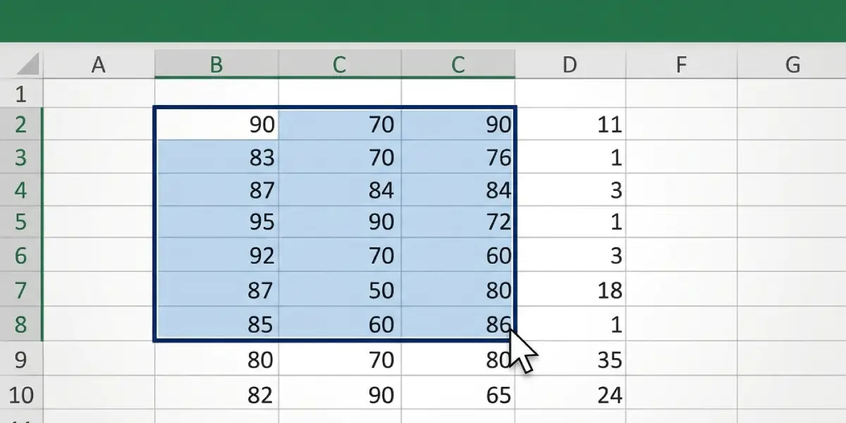
- Step 1: Open the workbook and select the range of cells to shade. Click the first cell and drag to the last, or click a column letter to select a whole column. Only numeric values are shaded, so headers can be included without harm, but leaving them out keeps things tidy.
- Step 2: Go to the Home tab on the ribbon.
- Step 3: In the Styles group, click Conditional Formatting.
- Step 4: Point to Color Scales in the dropdown menu. A gallery of presets appears.
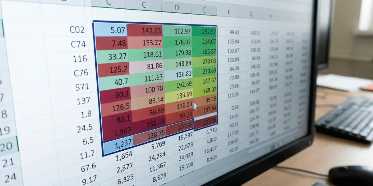
- Step 5: Hover over a preset to preview it on the selected cells. The preset names describe the color order. For example, Green – Yellow – Red Color Scale shades the highest values green, the middle values yellow, and the lowest values red.
- Step 6: Click the preset to apply it. The shading is applied instantly and updates automatically whenever the numbers change.
Tip: Most people find that a three-color scale works best for data with a natural midpoint, such as sales against a target, while a two-color scale is cleaner for plain low-to-high data like monthly totals.
Choosing Between Two-Color and Three-Color Presets
A two-color scale blends from one color to another, so it shows a simple gradient from the smallest to the largest value. A three-color scale adds a middle color at the 50th percentile, which makes it easier to spot which cells sit above or below the middle of the pack. Think of it like a thermometer: two colors show cold to hot, three colors also mark the comfortable middle.
How to Customize a Color Scale in Excel
The presets cover most needs, but colors and thresholds can be changed to match a report or a brand palette.
- Step 1: Select the range that already has a color scale applied.
- Step 2: Click Home, then Conditional Formatting, then Manage Rules.
- Step 3: Select the Color Scale rule in the list and click Edit Rule.
- Step 4: Under Edit the Rule Description, set the Type for the Minimum, Midpoint, and Maximum. Options include Lowest Value, Highest Value, Number, Percent, Formula, and Percentile.
- Step 5: Click the Color dropdown beside each point and choose a new color.
- Step 6: Click OK, then OK again in the Rules Manager to save the changes.
Tip: To build a new rule from scratch instead of editing a preset, choose Conditional Formatting > Color Scales > More Rules, then set the format style to 2-Color Scale or 3-Color Scale.
How to Remove a Color Scale in Excel
- Step 1: Select the shaded cells.
- Step 2: Click Home > Conditional Formatting > Clear Rules.
- Step 3: Choose Clear Rules from Selected Cells, or Clear Rules from Entire Sheet to remove all conditional formatting on the sheet.
Common Problems and Fixes
The Color Scale Option Is Greyed Out
This usually happens when the worksheet is protected or the file is open in a restricted view. Click Enable Editing if a yellow bar appears at the top, or go to Review > Unprotect Sheet and then try again.
Some Cells Are Not Shaded
Cells that contain numbers stored as text are skipped. A small green triangle in the corner of the cell is the usual sign. Select those cells, click the warning icon, and choose Convert to Number.
One Extreme Value Makes Every Other Cell Look the Same
A single very large number stretches the scale so the rest of the data looks almost identical in color. Open Manage Rules, edit the rule, and change the Minimum and Maximum Type to Percentile, such as the 10th and 90th, so outliers no longer dominate.
The Colors Do Not Change When Values Change
If shading looks frozen, check that calculation is not set to manual. Go to Formulas > Calculation Options and select Automatic.
The Scale Covers the Wrong Range
Open Conditional Formatting > Manage Rules, set Show formatting rules for to This Worksheet, and adjust the Applies to box for the rule so it matches the intended cells.
Frequently Asked Questions
Where is the color scale option in Excel?
It is on the Home tab, in the Styles group. Click Conditional Formatting, then point to Color Scales to see the presets.
Can a color scale be applied to a whole column?
Yes. Click the column letter to select the entire column, then apply the color scale from the Conditional Formatting menu. New numbers added to that column are shaded automatically.
What is the difference between a two-color and a three-color scale?
A two-color scale blends between a lowest-value color and a highest-value color. A three-color scale adds a midpoint color, which helps separate above-average from below-average values.
Can the colors in a color scale be changed?
Yes. Open Conditional Formatting > Manage Rules, select the color scale rule, click Edit Rule, and pick new colors for the minimum, midpoint, and maximum.
Does a color scale update when the data changes?
Yes. The shading recalculates automatically whenever a value in the range changes, as long as calculation is set to Automatic.
Why are some cells not colored by the scale?
Blank cells and numbers stored as text are ignored. Convert text-based numbers to real numbers and the shading will appear.
Can a color scale be applied to text?
No. Color scales only work on numeric values, including dates and times. Text entries are not shaded.
How can a color scale be removed?
Select the cells, then go to Home > Conditional Formatting > Clear Rules and choose Clear Rules from Selected Cells.
Can a color scale be applied to a PivotTable?
Yes. Select the value cells in the PivotTable and apply the color scale as usual. The Formatting Options button that appears lets the rule apply to all cells showing the same value field.