
Need to build a radar chart in Excel to compare skills, product scores, or survey results across several categories? The process takes only a few minutes once the data is laid out correctly. This guide walks through the exact clicks, from preparing the table to polishing the finished chart.
Key Takeaways
- Arrange categories in one column and each series in its own column, with headers in the top row.
- Select the full range, then use Insert, Charts, Waterfall or Stock or Radar, and pick Radar, Radar with Markers, or Filled Radar.
- Set the axis minimum and maximum so every series is judged on the same scale.
- Use Chart Design and Format Axis to tidy the title, legend, and gridlines.
Step-by-Step Guide to Build a Radar Chart in Excel
This works best when the data is small and comparable. Think of a radar chart as a spider web: each category is a spoke, and each series draws a shape across those spokes. Five to eight categories usually keep the web readable.
Prepare the Data
- Step 1: Open a worksheet and type the category names down the first column, starting in cell A2. For example, a skills review might list Communication, Teamwork, Technical Skill, Creativity, Leadership, and Time Management.
- Step 2: Type a header for each series across row 1, starting in cell B1. For example, B1 could read ‘Employee A’ and C1 could read ‘Employee B’.
- Step 3: Enter the numeric scores in the cells under each header. Keep all values on the same scale, such as 1 to 10, so the shapes compare fairly.
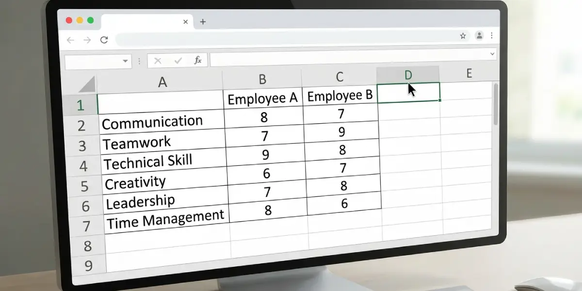
Tip: Leave cell A1 blank. Excel then treats the first column as category labels and the first row as series names, which avoids a common mix-up where the labels get plotted as a data series.
Insert the Radar Chart
- Step 4: Click any cell inside the data table, or drag to select the whole range including the headers and category names.
- Step 5: Go to the Insert tab on the ribbon.
- Step 6: In the Charts group, click the Insert Stock, Surface or Radar Chart button. In some versions this button is labeled Insert Waterfall, Funnel, Stock, Surface or Radar Chart.
- Step 7: Under Radar, choose Radar, Radar with Markers, or Filled Radar. Radar with Markers is a solid pick when comparing two or three series, because the dots make each score easy to spot.
- Step 8: The chart appears on the worksheet. Drag it to a clear spot and resize it using the corner handles.
Tip: Filled Radar looks bold, but the top series can hide the ones behind it. When comparing more than two series, Radar with Markers is usually the clearer choice.
Format the Radar Chart
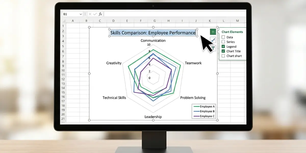
- Step 9: Click the chart title and type a descriptive name, such as ‘Skills Comparison by Employee’. To remove the title, select the chart, click the Chart Elements plus icon beside it, and clear the Chart Title box.
- Step 10: Right-click the numbers running along the vertical axis and select Format Axis. In the Axis Options pane, set Minimum to 0 and Maximum to the top of the scale, such as 10.
- Step 11: In the same pane, set the Major unit to 2 for a cleaner grid, for instance, if the scale runs from 0 to 10.
- Step 12: Select the chart, then open the Chart Design tab and click Change Colors or pick a Chart Style to match the document or presentation.
- Step 13: Click the Chart Elements plus icon and tick Legend so each colored line can be traced to its series. Use the arrow next to Legend to place it at the bottom or right.
- Step 14: To change one series line, click that line on the chart, right-click, and choose Format Data Series. Adjust the line color, width, or marker style under the Fill and Line section.
Common Problems and Fixes
The Radar Chart Option Is Greyed Out
This usually happens when no data is selected or the selection is a single cell with no neighboring numbers. Click inside the table first, confirm it holds numeric values, and open the Insert tab again.
Categories Appear as a Data Series
When cell A1 contains text, Excel may treat the first column as a series instead of labels. Clear cell A1, then right-click the chart, choose Select Data, and confirm the category names appear under Horizontal (Category) Axis Labels.
The Shapes Look Tiny or Squashed
Excel picks the axis scale automatically, and an odd maximum can shrink the shapes. Right-click the vertical axis, choose Format Axis, and set a fixed Minimum and Maximum that match the data range.
Rows and Columns Are Flipped
If each spoke shows a series instead of a category, the data orientation is reversed. Click the chart, open the Chart Design tab, and select Switch Row/Column.
Category Labels Are Cut Off or Overlapping
Long names crowd the edges of the web. Shorten the labels in the worksheet, or drag the chart wider so the text has room to breathe.
The Chart Shows Zero for Blank Cells
Empty cells plot as gaps or zeros, which distorts the shape. Fill every cell with a real score, or enter 0 on purpose so the chart reflects the intended value.
Frequently Asked Questions
Where is the radar chart option in Excel?
Select the data, open the Insert tab, and in the Charts group click the Insert Stock, Surface or Radar Chart button. The Radar, Radar with Markers, and Filled Radar options are listed there.
How many categories should a radar chart have?
Between five and eight categories keeps the chart readable. More spokes crowd the labels and make the shapes harder to compare.
Can a radar chart in Excel show more than one series?
Yes. Put each series in its own column with a header, select the full range, and insert the chart. Each series appears as a separate colored line or shape.
How do I change the scale of a radar chart?
Right-click the numbers on the vertical axis, select Format Axis, and set the Minimum, Maximum, and Major unit values in the Axis Options pane.
How do I add or remove the legend?
Click the chart, select the Chart Elements plus icon, and tick or clear the Legend box. The arrow beside it controls where the legend sits.
Why does my radar chart look wrong after inserting it?
The most common causes are a filled cell A1, rows and columns reversed, or blank cells in the data. Use Switch Row/Column on the Chart Design tab and check that every cell holds a value.
Can the chart title be edited or removed?
Yes. Click the title and type new text to edit it. To remove it, use the Chart Elements plus icon and clear the Chart Title box.
How do I change the color of a series in a radar chart?
Click the series line on the chart, right-click, and choose Format Data Series. Under Fill and Line, pick a new color. The Change Colors button on the Chart Design tab recolors every series at once.