
Need to add data labels from cell values in Excel instead of showing the default numbers? The Value From Cells option lets any chart label pull its text straight from a range on the worksheet. It works well for product names, status notes, percentages, or any custom text sitting next to the data.
Key Takeaways
- The feature is called Value From Cells and is found in the Format Data Labels pane.
- The label range must be selected separately from the chart data, and it should match the number of data points.
- Untick Value or Y Value if only the cell text should appear on the chart.
- Labels update automatically when the linked cells change.
- The option is available in Excel 2013 and later, including Microsoft 365.
Step-by-Step Guide to Add Data Labels From Cell Values in Excel
This works best when the chart already exists and the label text is typed or calculated in a column or row next to the source data. Picture a sales chart where each bar needs a short note such as ‘Launch month’ or ‘Top seller’. Those notes live in a helper column, and the steps below connect them to the bars.
Prepare the Label Range
- Step 1: Type or calculate the label text in a block of cells next to the chart data. Keep the same number of cells as there are data points in the series, in the same order.
- Step 2: Click the chart once to select it. The Chart Design and Format tabs appear on the ribbon.
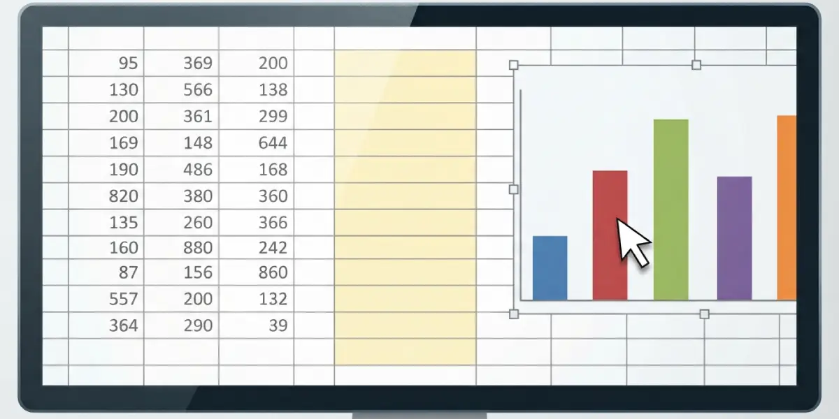
Turn On Value From Cells
- Step 3: Click the Chart Elements button, the green plus sign at the top right of the chart, and tick the Data Labels check box. On Mac, go to Chart Design, then Add Chart Element, then Data Labels.
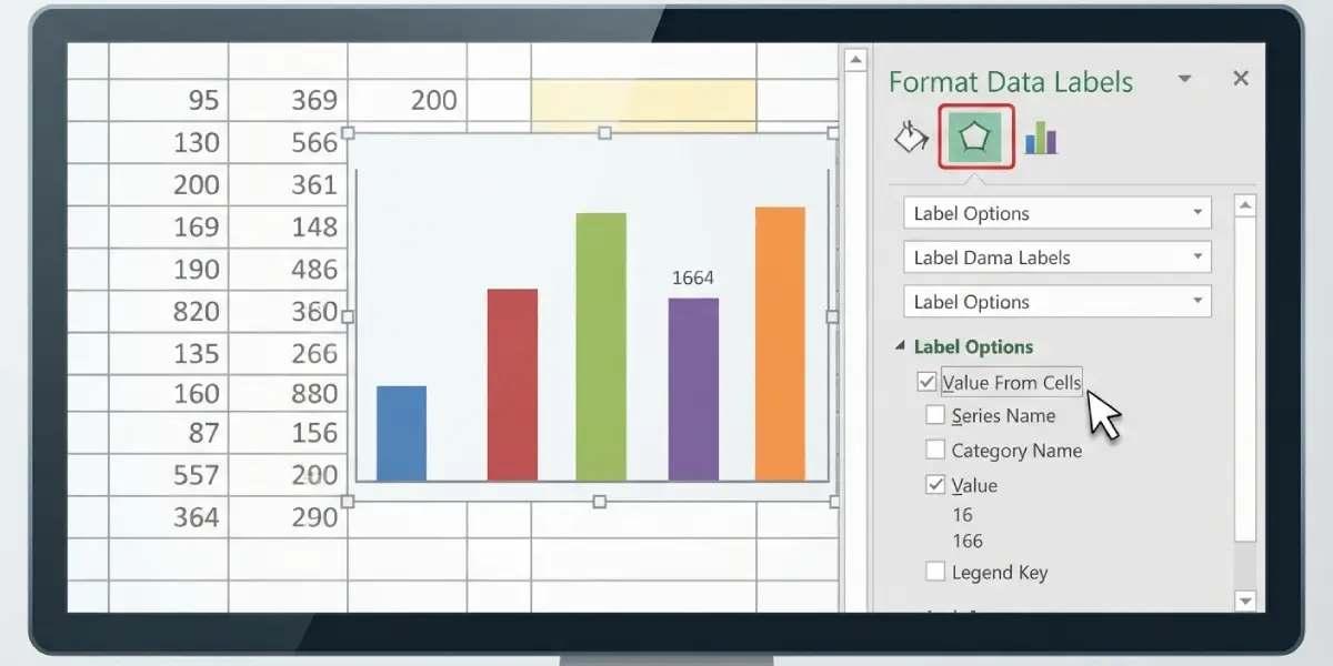
- Step 4: Click the small arrow next to Data Labels and choose More Options (on Mac, More Data Label Options). The Format Data Labels pane opens on the right.
- Step 5: In the pane, select the Label Options icon, which looks like a small bar chart, and expand the Label Options section.
- Step 6: Tick the Value From Cells check box. The Data Label Range dialog box appears.
- Step 7: Click the range selector, drag across the label cells on the worksheet, and press OK.
- Step 8: Under Label Contains, untick Value (or Y Value on scatter and line charts) if the chart should show only the cell text. Leave it ticked to display both the number and the text.
Tip: Choose a separator such as a comma, new line, or space in the Separator list when both the value and the cell text are shown. A new line keeps labels tidy on narrow columns.
Position and Check the Labels
- Step 9: Under Label Position in the same pane, pick Outside End, Inside End, Center, or another option that fits the chart type.
- Step 10: Change one of the linked cells and confirm that the matching label updates on the chart.
Tip: Use a formula such as =B2&’ – ‘&C2 in the label column to combine two columns into one label. The chart label follows the formula result.
Common Problems and Fixes
The Value From Cells Option Is Missing
This option was introduced in Excel 2013, so Excel 2010 and earlier do not have it. In a newer version, make sure a data label is actually selected and the Format Data Labels pane is open, not the Format Chart Area pane.
Labels Show Numbers Instead of the Cell Text
The Value or Y Value box is still ticked, so numbers appear alongside or instead of the text. Untick it under Label Contains in the Format Data Labels pane.
Labels Appear on the Wrong Points
The label range is probably in a different order than the chart data, or it has a different number of cells. Reopen Value From Cells, reselect the range, and confirm it lines up with the series.
Labels Show Brackets Like [CELLRANGE]
This placeholder appears when the linked range is lost or the label has been edited manually. Reselect Value From Cells and choose the range again to restore the link.
Only One Series Has Cell-Based Labels
Data labels are set per series. Click a label from the other series and repeat the steps with its own label range.
Frequently Asked Questions
Which Excel versions support data labels from cell values?
Excel 2013 and later support the Value From Cells option, including Excel 2016, 2019, 2021, and Microsoft 365. Excel 2010 and earlier do not include it.
Where is the Value From Cells option located?
It is in the Format Data Labels pane, under Label Options, in the Label Contains section. Open the pane by choosing Data Labels, then More Options, from the Chart Elements button.
Can the label range be on a different worksheet?
Yes. In the Data Label Range dialog box, switch to the other sheet and select the cells. The labels continue to update when those cells change.
Do the labels update when the cell text changes?
Yes. The labels are linked to the cells, so any edit or formula result change appears on the chart automatically.
How can the chart show only the cell text and not the number?
After ticking Value From Cells, untick Value (or Y Value) under Label Contains. Only the text from the selected range remains.
Does the label range need the same number of cells as the data points?
It should. A matching count and order make sure each label lands on the correct point. A shorter range leaves some points without labels.
Can data labels from cell values be used on every chart type?
Value From Cells works on most common chart types, including column, bar, line, scatter, and bubble charts. It is especially useful on scatter and bubble charts, where points have no names by default.
How can the cell-based labels be removed?
Open the Format Data Labels pane and untick Value From Cells. To remove all labels, untick Data Labels in the Chart Elements menu.