
Using Excel VLOOKUP with multiple criteria sounds impossible at first, because VLOOKUP only searches for one value at a time. The fix is simple: combine the criteria into a single lookup value, then let VLOOKUP find it. This guide uses a sales table where the goal is to pull a revenue figure based on both a Region and a Product.
Key Takeaways
- VLOOKUP can only match one value, so multiple criteria must be joined into one with the & operator.
- A helper column placed to the left of the data holds the combined key for every row.
- The lookup formula joins the same criteria and searches the helper column with FALSE for an exact match.
- A one-formula option using CHOOSE avoids the helper column entirely.
- Most errors come from extra spaces, mismatched data types, or a wrong column number.
How to Use VLOOKUP with Multiple Criteria in Excel
The example below assumes a table with Region in column B, Product in column C, Sales Rep in column D, and Revenue in column E. Column A is empty and will hold the helper formula. The two lookup criteria are typed into H2 (Region) and I2 (Product), and the result will appear in J2.
Build the Helper Column
- Step 1: Make sure the column to the left of the data is empty. If the table starts in column A, right-click the column A header and choose Insert to add a new blank column. VLOOKUP can only return values from columns to the right of the lookup column, so the helper must come first.
- Step 2: Type a heading such as Key in cell A1.
- Step 3: In cell A2, enter the formula =B2&C2 and press Enter. This joins the Region and Product into one text value, for example EastLaptop.
- Step 4: Double-click the fill handle (the small square at the bottom-right corner of A2) to copy the formula down to the last row of data.
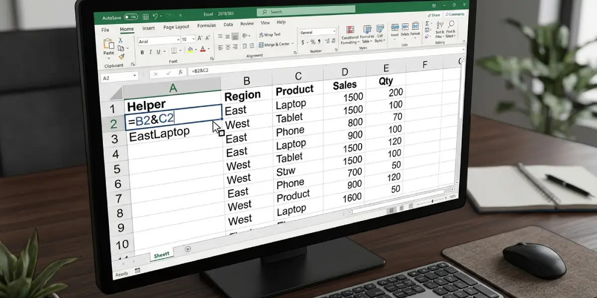
Tip: Hide the helper column once the formulas are in place. Right-click the column A header and choose Hide. Hidden columns still work perfectly in VLOOKUP.
Write the Lookup Formula
- Step 5: Enter the Region to find in H2 and the Product to find in I2.
- Step 6: Click cell J2 and type =VLOOKUP(H2&I2,$A$2:$E$100,5,FALSE) and press Enter.
- Step 7: Check the result. The formula joins H2 and I2 into one value, searches column A of the range for that exact key, and returns the matching value from the fifth column of the range, which is Revenue.
- Step 8: Change the values in H2 or I2 to confirm the result updates correctly.
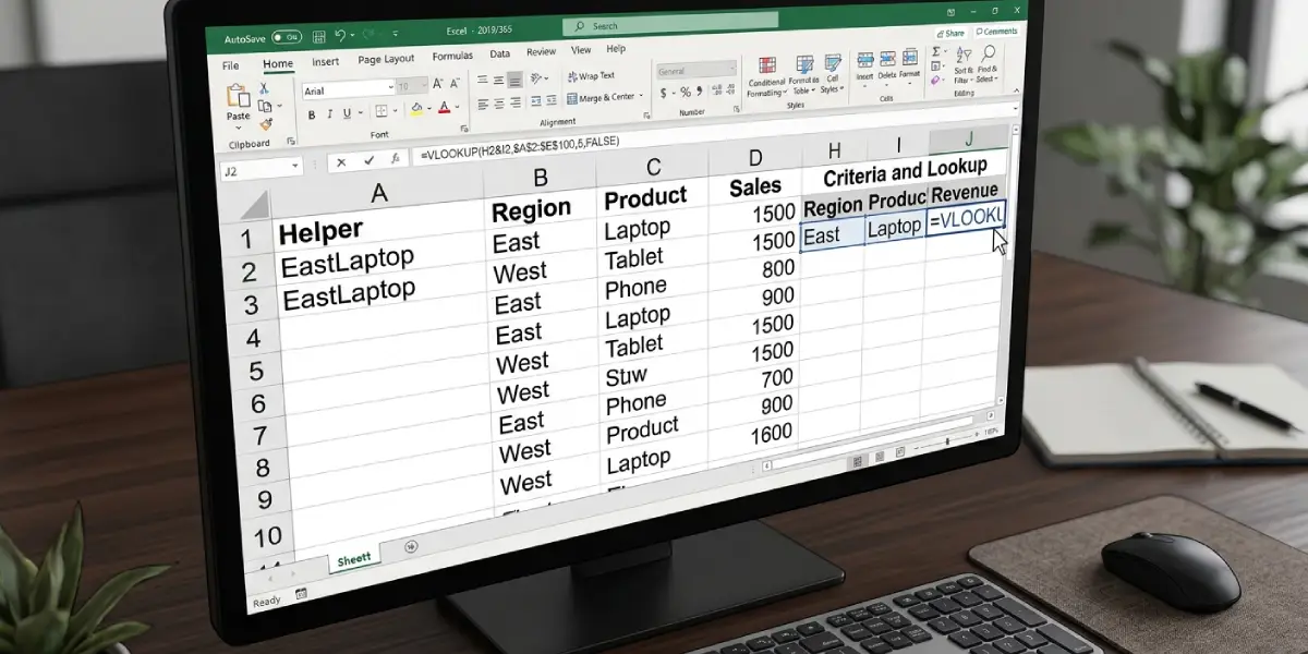
Tip: Lock the table range with dollar signs, as in $A$2:$E$100, so the range does not shift when the formula is copied to other cells.
Add More Than Two Criteria
- Step 9: To match three criteria, extend both sides of the formula. For example, make the helper formula =B2&C2&D2, then use =VLOOKUP(H2&I2&K2,$A$2:$E$100,5,FALSE), where K2 holds the third criterion. The order of the joined values must be identical in the helper column and in the lookup.
Using VLOOKUP with Multiple Criteria Without a Helper Column
When adding a column is not possible, the CHOOSE function can build the combined key inside the formula itself. This works best when the sheet layout cannot be changed.
- Step 1: Click the cell where the result should appear, such as J2.
- Step 2: Enter =VLOOKUP(H2&I2,CHOOSE({1,2},B2:B100&C2:C100,E2:E100),2,FALSE).
- Step 3: Press Enter in Microsoft 365 or Excel 2021 and later. In older versions, press Ctrl+Shift+Enter so the formula is entered as an array formula.
The CHOOSE part builds a temporary two-column table in memory. The first column is the combined Region and Product, and the second is Revenue, which is why the column number is 2.
Common Problems and Fixes
The Formula Returns #N/A
This usually means no exact match was found. Check for stray spaces in the source data or in the criteria cells. Wrapping the pieces in TRIM, such as =TRIM(B2)&TRIM(C2), removes hidden spaces. Also confirm that the helper column and the lookup formula join the criteria in the same order.
The Formula Returns the Wrong Value
The last argument must be FALSE. Leaving it out or using TRUE switches VLOOKUP to approximate matching, which can return a nearby but incorrect row.
The Formula Returns #REF!
The column number is larger than the number of columns in the selected range. If the range is A2:E100, the highest valid column number is 5.
The Result Shows Revenue from the Wrong Column
The column number counts from the first column of the range, which is the helper column. Revenue in column E of a range starting at column A is column number 5, not 4.
The Formula Appears as Text Instead of a Result
The cell is probably formatted as Text. Change the format to General on the Home tab, then click into the cell and press Enter again.
Numbers Do Not Match
Joining values with & turns everything into text. If the criteria are numbers in some places and text in others, the keys will not match. Make sure both the helper column and the lookup cells use the same kind of data.
Frequently Asked Questions
Can VLOOKUP really use more than one criterion?
Not directly. VLOOKUP accepts a single lookup value, so the criteria must be combined into one value first, either with a helper column or with CHOOSE inside the formula.
Why does the helper column have to be on the left?
VLOOKUP always searches the first column of the selected range and can only return values from columns to its right. The combined key must therefore be the first column in the range.
How many criteria can be combined?
There is no practical limit. Keep joining values with the & operator in both the helper column and the lookup formula, as long as the order is identical.
Does this work in older versions of Excel?
The helper column method works in every version of Excel. The CHOOSE method works in all versions too, but versions before Excel 2021 require pressing Ctrl+Shift+Enter to confirm the formula.
What happens if two rows share the same combined key?
VLOOKUP returns the first match from top to bottom and ignores the rest. If duplicates exist, the data may need an additional criterion to make each key unique.
Is the lookup case-sensitive?
No. VLOOKUP treats uppercase and lowercase letters as the same, so East and EAST produce the same match.
Why does the formula work in one cell but fail when copied down?
The table range is probably not locked. Use absolute references like $A$2:$E$100 so the range stays fixed while the lookup criteria cells change.
Can the helper column be deleted after the lookup works?
No. The lookup formula depends on the helper column, so deleting it breaks the result. Hide the column instead if it clutters the sheet.