
Fixing the #N/A error in Excel fast comes down to one thing: Excel searched for a value and could not find a match. This guide walks through the exact checks that clear it, in the order that solves the most cases with the least effort. Every step below works in Excel for Microsoft 365, Excel 2021, Excel 2019, and Excel for the web.
Key Takeaways
- #N/A always means the lookup value was not found – it is not a broken formula, it is a failed search.
- Most cases are caused by hidden spaces, numbers stored as text, or an approximate match left switched on.
- Confirm the value really exists with COUNTIF before changing anything else.
- TRIM and VALUE fix the two most common data mismatches in under a minute.
- Wrap the finished formula in IFNA only after the real cause is corrected, never before.
Step-by-Step Guide to Fixing the #N/A Error in Excel Fast
Work through these steps in order. The cause is usually found by step four, so there is rarely any need to go further.
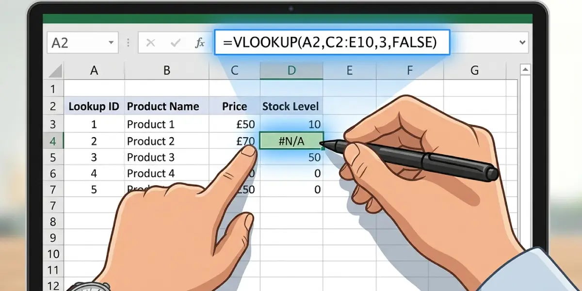
- Step 1: Click the cell showing #N/A and read the formula in the formula bar. Note the lookup value (the first argument) and the range being searched. Functions that produce #N/A include VLOOKUP, HLOOKUP, XLOOKUP, LOOKUP, MATCH, and anything built on INDEX and MATCH.
- Step 2: Hover over the small warning triangle beside the cell, or select the cell and go to Formulas, then Error Checking. Excel names the argument it could not resolve, which points straight at the problem column.
- Step 3: Test whether the value genuinely exists. In an empty cell, enter =COUNTIF(D:D,A2) where D:D is the column being searched and A2 holds the lookup value. A result of 0 means Excel sees no match; a result of 1 or more means the values differ in format, not in content.
- Step 4: Strip out stray spaces. Trailing spaces from pasted reports are the single most common cause of #N/A. In a helper column, enter =TRIM(A2), copy the results, then use Paste Special and Values to replace the original column. Do the same on the lookup column if needed.
- Step 5: Match the data types. A product code typed as 00451 in one sheet and 451 in another will never match. Select the column, open Data, then Text to Columns, click Finish, and Excel re-evaluates the entries. For the reverse direction, =VALUE(A2) converts text digits into real numbers.
- Step 6: Force an exact match. In VLOOKUP and HLOOKUP, the final argument must be FALSE (or 0). Leaving it blank tells Excel to accept the nearest lower value, which fails loudly on unsorted data. XLOOKUP is exact by default, so no change is needed there.
- Step 7: Check the search direction. VLOOKUP only looks in the first column of the table array, so if the lookup value sits to the right of the answer, the search cannot succeed. Either move the column or switch to XLOOKUP, which searches any column in any direction.
- Step 8: Lock the range before copying the formula down. Change B2:C500 to $B$2:$C$500 by pressing F4 while the reference is selected. Unlocked ranges slide down the sheet as the formula is filled, leaving later rows searching empty cells.
- Step 9: Recalculate and confirm. Press F9, then check a few rows near the top, middle, and bottom of the column rather than only the first result.
- Step 10: Handle the legitimate blanks. Once the real errors are gone, any remaining #N/A means the item truly is missing. Wrap the formula as =IFNA(VLOOKUP(A2,$B$2:$C$500,2,FALSE),0) to return 0, or replace the 0 with your own message inside quotation marks.
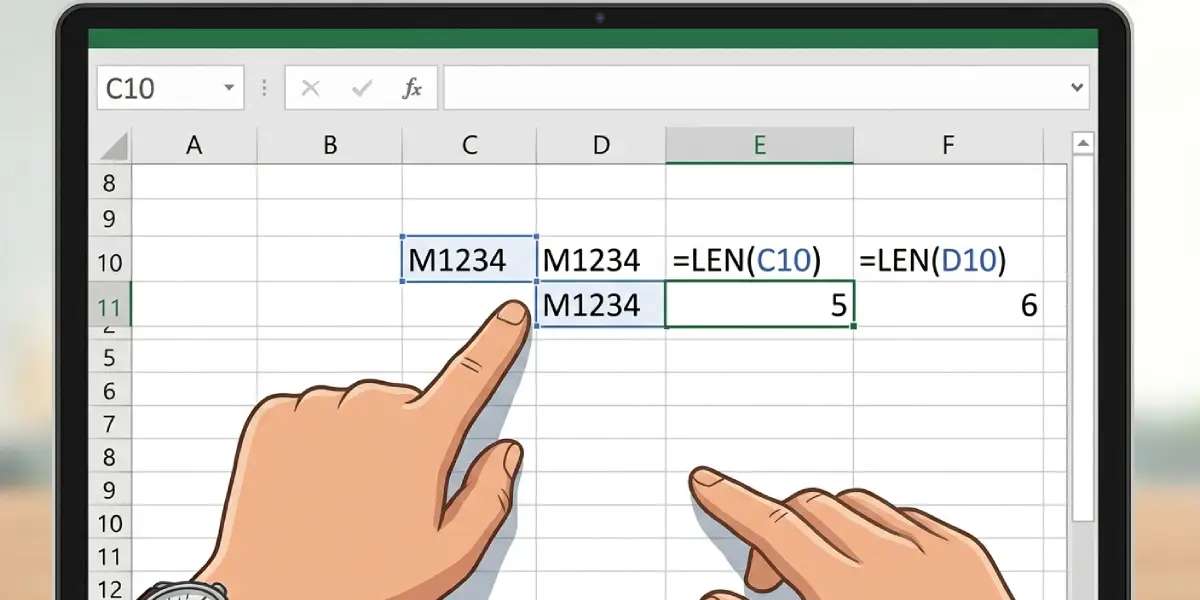
A quick way to see the hidden character
When COUNTIF returns 1 but the lookup still fails, put =LEN(A2) next to =LEN(D2). If one shows 7 and the other shows 8, there is an invisible character in the longer entry. This trick takes ten seconds and settles the argument immediately.
Tip: Non-breaking spaces copied from web pages and PDFs survive TRIM. Use =TRIM(SUBSTITUTE(A2,CHAR(160),CHAR(32))) to clear those as well, then paste the result back as values.
When the source data lives in another workbook
Lookups pointing at a closed workbook return #N/A rather than the expected result in some functions. Open the source file, press F9, and the values resolve. Most people find that copying the needed range into the same workbook is faster and far more stable for anything that gets shared by email.
Common Problems and Fixes
COUNTIF says the value exists but the lookup still fails
COUNTIF ignores some formatting differences that lookup functions respect. Run the LEN comparison described above, then apply TRIM and Text to Columns to both columns so they end up in the same format.
The first row works and every row below it breaks
This is the classic unlocked reference problem. Press F4 on the table array to add dollar signs, or convert the source range to a table through Insert, then Table, so the reference stays anchored automatically.
TRIM was applied but nothing changed
The TRIM result was probably left sitting in the helper column while the formula still points at the original. Copy the helper column, right-click the original, choose Paste Special, and select Values before deleting the helper.
MATCH returns #N/A inside an INDEX formula
The failure is in MATCH, not INDEX. Check that the third argument of MATCH is 0 for an exact match, and that the lookup array is a single row or column rather than a block of cells.
Dates refuse to match
One column holds real dates and the other holds text that merely looks like a date. Select the text column, run Text to Columns, and on the third screen choose Date with the correct order, such as DMY or MDY.
The error returned after the file was reopened
Calculation is likely set to Manual. Go to Formulas, then Calculation Options, and select Automatic.
IFNA hides the error but the numbers look wrong
IFNA only masks the symptom. If totals are lower than expected, remove the IFNA wrapper temporarily, fix the underlying mismatches with steps four through seven, then put the wrapper back.
Frequently Asked Questions
What does the #N/A error actually mean in Excel?
It means ‘not available’ – Excel ran the search and found no matching value. The formula itself is valid, so the fix belongs in the data or in the match settings rather than in the formula structure.
What is the fastest way to fix #N/A in a VLOOKUP?
Set the last argument to FALSE, then apply TRIM to both the lookup value and the first column of the table array. That pair of changes resolves the large majority of VLOOKUP cases.
Should IFERROR or IFNA be used to clear the error?
IFNA is the safer choice because it only traps #N/A. IFERROR swallows every error type, including #REF and #VALUE, which can hide genuine problems such as a deleted column.
Why does the lookup fail when both cells look identical?
One entry almost certainly contains a trailing space, a non-breaking space, or digits stored as text. Compare the two with LEN to confirm, then clean the longer entry.
Does XLOOKUP prevent the #N/A error?
XLOOKUP still returns #N/A when no match exists, but it defaults to exact matching and accepts an if_not_found argument directly, so fewer errors appear in the first place.
Can #N/A be removed without changing the formula?
Yes. Correcting the source data – trimming spaces, converting text to numbers, or adding the missing record – clears the error while the formula stays exactly as written.
Why do some rows show #N/A after copying a formula down?
The table array is unlocked and shifts with each row. Add dollar signs with F4, or use a structured table reference so the range never moves.
Will hiding #N/A affect SUM or AVERAGE results?
An unhandled #N/A spreads to any formula that references it, so SUM and AVERAGE will also return #N/A. Wrapping the lookup in IFNA with a 0 restores normal aggregation.
Does Find and Replace work for removing #N/A?
Not on formula results, since the cell contains a formula rather than the text #N/A. It works only where the errors were pasted in as static values.
Is #N/A ever the correct result to keep?
Often, yes. In reconciliation and audit work, a visible #N/A flags a record that is genuinely missing from the source, which is more useful than a silent zero.