
Need to show how a starting number grows or shrinks to reach a final result? The quickest way to build a waterfall chart in Excel is to lay out your data in two columns, insert the built-in Waterfall chart, and mark any totals. The whole process takes only a few minutes in Excel 2016 or later and Microsoft 365.
Key Takeaways
- A waterfall chart needs just two columns: labels and values, with negative numbers for decreases.
- The built-in Waterfall option is found on the Insert tab in Excel 2016 and later.
- Starting and ending bars must be set as totals so they anchor to the baseline.
- Data labels, colors, and connector lines can be adjusted from the Chart Design tab and the Format pane.
Step-by-Step Guide to Build a Waterfall Chart in Excel
Prepare the Data
A clean layout makes everything else easier. Think of the data like a bank statement: an opening balance, a list of deposits and withdrawals, and a closing balance.
- Step 1: Type the category labels in column A, such as ‘Starting Balance’, ‘Sales’, ‘Refunds’, ‘Shipping’, and ‘Ending Balance’.
- Step 2: Enter the matching values in column B. Use positive numbers for increases and negative numbers for decreases, for example 5000, 3200, -450, -800.
- Step 3: Add the ending value in the last row if it should appear as its own total bar. Enter the final calculated amount there, either typed in or with a formula such as =SUM(B2:B5).
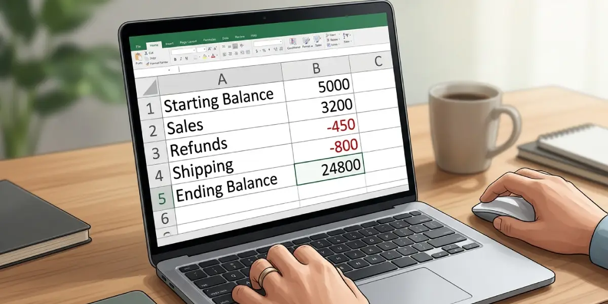
Tip: Add a header row with names like ‘Item’ and ‘Amount’. Excel then reads the first row as headers and not as chart data.
Insert the Waterfall Chart
- Step 4: Click any cell inside the data range, or select the whole range including headers.
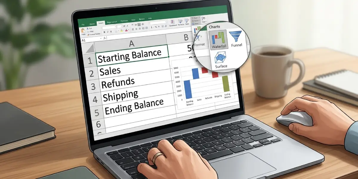
- Step 5: Go to the Insert tab on the ribbon.
- Step 6: In the Charts group, click the ‘Insert Waterfall, Funnel, Stock, Surface, or Radar Chart’ icon.
- Step 7: Under the Waterfall heading, choose ‘Waterfall’. The chart appears on the worksheet with increases, decreases, and totals shown in different colors.
Set the Totals
At first, every bar floats from the previous one, including the opening and closing values. This is the step most people miss. The key is to tell Excel which bars are totals so they start from zero.
- Step 8: Click once on the first bar to select the whole data series, then click the bar again to select only that single data point.
- Step 9: Right-click the bar and choose ‘Set as Total’. The bar drops to the baseline and takes on the Total color.
- Step 10: Repeat for the ending bar and for any subtotal bar in the middle of the data.
Tip: To reverse the change, right-click the same bar and select ‘Set as Total’ again to toggle it off.
Format the Chart
- Step 11: Click the chart title and type a clear name, such as ‘Monthly Cash Flow’.
- Step 12: Select the chart, open the Chart Design tab, click Add Chart Element, point to Data Labels, and pick a position to show the value on each bar.
- Step 13: Right-click any bar and choose ‘Format Data Series’ to open the Format pane. Adjust the Gap Width to make the bars thicker or thinner, and turn ‘Show connector lines’ on or off.
- Step 14: To change colors, click a legend entry such as Increase, Decrease, or Total, then use the Fill option in the Format pane or on the Format tab.
Common Problems and Fixes
The Waterfall Option Is Missing or Greyed Out
This chart type is not available in Excel 2013 or earlier. It also stays unavailable if the workbook is saved in the older .xls format. Save the file as .xlsx and reopen it, or use a version of Excel from 2016 onward.
The First or Last Bar Floats Instead of Starting at Zero
The bar has not been marked as a total. Right-click it and select ‘Set as Total’.
The Ending Bar Is Counted Twice
When the final total is entered as a regular value and not set as a total, Excel adds it to the running balance. Mark that bar as a total so it is shown as the sum and not added again.
Data Labels Show Too Many Decimals
Right-click a data label, choose ‘Format Data Labels’, expand Number, and select a category such as Number or Currency with the decimal places needed.
Categories Appear in the Wrong Order
The chart follows the row order of the source data. Reorder the rows in the worksheet and the chart updates automatically.
Frequently Asked Questions
Which versions of Excel can create a waterfall chart?
Excel 2016 and later, including Microsoft 365 and Excel for Mac 2016 or later, include the built-in Waterfall chart. Earlier versions do not have it.
Where is the waterfall chart option in Excel?
Open the Insert tab, go to the Charts group, click the ‘Insert Waterfall, Funnel, Stock, Surface, or Radar Chart’ icon, and select Waterfall.
How should the data be arranged for a waterfall chart?
Place labels in one column and values in the next. Use positive numbers for increases and negative numbers for decreases, with the starting and ending values in the first and last rows.
How do I make a bar start from zero?
Click the bar twice to select that single point, right-click it, and choose ‘Set as Total’. The bar then anchors to the baseline.
Can a waterfall chart include subtotals?
Yes. Add a subtotal row in the data, then right-click its bar and choose ‘Set as Total’. The chart treats it as a new baseline bar.
How do I change the colors of increases and decreases?
Click the matching legend entry, such as Increase, Decrease, or Total, and apply a new fill color from the Format pane or the Format tab.
How do I add data labels to a waterfall chart?
Select the chart, go to the Chart Design tab, click Add Chart Element, choose Data Labels, and select a position. The values then appear on each bar.
How do I remove the connector lines between bars?
Right-click a bar, choose ‘Format Data Series’, and uncheck ‘Show connector lines’ in the Series Options.