
If a VLOOKUP formula keeps breaking whenever a column is inserted, it is time to use XLOOKUP instead of VLOOKUP in Excel. XLOOKUP needs no column index number, looks in any direction, and returns an exact match by default. The steps below convert a typical VLOOKUP into XLOOKUP in a couple of minutes.
Key Takeaways
- XLOOKUP uses the syntax =XLOOKUP(lookup_value, lookup_array, return_array), so no column index number is needed.
- It finds exact matches by default, so there is no FALSE argument to remember.
- It can return a value from a column to the left of the lookup column, which VLOOKUP cannot do.
- A built-in if_not_found argument replaces the IFERROR wrapper often wrapped around VLOOKUP.
- XLOOKUP is available in Excel for Microsoft 365, Excel 2021, Excel 2024, and Excel for the web.
Step-by-Step: Use XLOOKUP Instead of VLOOKUP in Excel
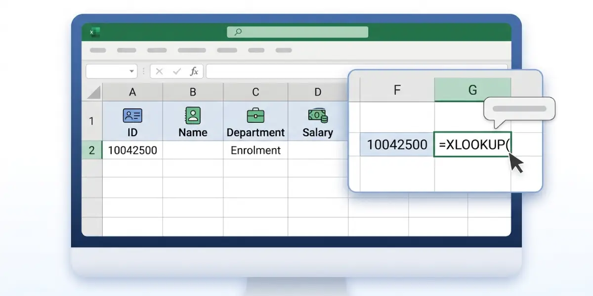
The example below uses an employee table in A1:D101, with Employee ID in column A, Name in B, Department in C, and Salary in D. The ID to search for is typed in cell F2. The old formula looked like this: =VLOOKUP(F2,A2:D101,3,FALSE). The goal is to return the same department using XLOOKUP.
- Step 1: Confirm the Excel version supports the function. Type =XLOOKUP( in any empty cell. If Excel shows the argument tooltip, the function is available. If it shows a #NAME? error, the version is too old (Excel 2019 and earlier do not include XLOOKUP).
- Step 2: Click the cell where the result should appear, for example G2.
- Step 3: Type =XLOOKUP( to start the formula.
- Step 4: Enter the lookup_value, which is the item being searched for. Click cell F2, then type a comma.
- Step 5: Enter the lookup_array, which is the single column that contains the item. Select A2:A101 and type a comma. Only the lookup column is selected here, not the whole table.
- Step 6: Enter the return_array, which is the single column holding the answer. Select C2:C101. This replaces the old column index number 3.
- Step 7: Close the bracket and press Enter. The finished formula reads =XLOOKUP(F2,A2:A101,C2:C101) and returns the department for the ID in F2.
- Step 8: Optionally add a fallback result as the fourth argument. For a salary lookup, =XLOOKUP(F2,A2:A101,D2:D101,0) returns 0 instead of #N/A when the ID does not exist. Text can also be used as the fallback, as long as it is typed between quotation marks.
- Step 9: Copy the formula down. Double-click the fill handle at the bottom-right corner of the cell, or drag it down. Lock the arrays with dollar signs (for example $A$2:$A$101) when copying the formula to other rows or columns so the ranges do not shift.
Tip: Select the lookup and return columns by clicking the column headers inside an Excel Table, or convert the data to a Table first (Ctrl + T). The formula then uses structured references and expands automatically when new rows are added.
Converting an Existing VLOOKUP Formula
Take =VLOOKUP(F2,A2:D101,3,FALSE). Each part maps directly to XLOOKUP:
- The first argument, F2, stays the same and becomes the lookup_value.
- The first column of the table range, A2:A101, becomes the lookup_array.
- The column picked by the index number 3, which is C2:C101, becomes the return_array.
- The FALSE argument is dropped because exact match is already the default.

The result is =XLOOKUP(F2,A2:A101,C2:C101), which does exactly the same job.
XLOOKUP Examples That VLOOKUP Cannot Handle Easily
Once the basic swap works, a few common situations show why this function is worth using. Each example uses the same employee table.
Look Up a Value to the Left
VLOOKUP only returns data from columns to the right of the lookup column. To find an Employee ID from a name typed in G2, use =XLOOKUP(G2,B2:B101,A2:A101). The return column sits to the left of the lookup column, and the formula works without any rearranging.
Return Several Columns at Once
To pull Name, Department, and Salary for one ID in a single formula, point the return_array at several columns: =XLOOKUP(F2,A2:A101,B2:D101). The results spill into the cells to the right automatically, so the cells next to the formula must be empty.
Find the Closest Smaller Value
This is useful for commission rates, tax bands, or grade boundaries. With thresholds in J2:J6 and rates in K2:K6, the formula =XLOOKUP(E2,J2:J6,K2:K6,0,-1) returns the rate for the highest threshold that does not exceed the value in E2. The fifth argument, -1, means exact match or the next smaller item. Using 1 instead returns the next larger item.
Return the Last Match Instead of the First
When an ID appears more than once, for example in a transaction log, add 1 as the sixth argument position by skipping the fifth: =XLOOKUP(F2,A2:A101,D2:D101,0,0,-1). The final -1 tells Excel to search from the bottom up, so the most recent entry is returned.
Tip: The optional arguments must stay in order: if_not_found, match_mode, then search_mode. To use a later argument without an earlier one, leave the earlier slot empty between commas.
Common Problems and Fixes
The Formula Returns #N/A
The lookup value was not found. Check for extra spaces, mismatched spelling, or numbers stored as text in one column and as real numbers in the other. Clean the data, or add the if_not_found argument so a friendly result appears instead of the error.
The Formula Returns #NAME?
This appears in versions of Excel that do not include XLOOKUP, such as Excel 2019, 2016, or earlier. It can also appear if the function name is mistyped. Check the spelling first, then confirm the version under File, Account, About Excel.
The Formula Returns #VALUE!
The lookup_array and return_array must be the same size. A mismatch such as A2:A101 against C2:C100 causes this error. Re-select both ranges so they have the same number of rows.
The Formula Returns #SPILL!
This happens when the return_array covers several columns and something is already sitting in the cells where results should spill. Clear the blocked cells, or shrink the return_array to a single column.
The Result Is Wrong After Copying the Formula Down
Ranges are shifting because they are not locked. Press F4 while the cursor is on each range to add dollar signs, so the lookup and return arrays stay fixed while the lookup value changes row by row.
Frequently Asked Questions
Is XLOOKUP better than VLOOKUP in Excel?
For most tasks, yes. XLOOKUP does not need a column index number, defaults to exact match, can look to the left, and has a built-in not-found argument. VLOOKUP still works, but breaks more easily when columns are inserted or deleted.
Which versions of Excel have XLOOKUP?
XLOOKUP is included in Excel for Microsoft 365, Excel 2021, Excel 2024, and Excel for the web. It is not available in Excel 2019, Excel 2016, or earlier versions.
What is the XLOOKUP syntax?
The syntax is =XLOOKUP(lookup_value, lookup_array, return_array, [if_not_found], [match_mode], [search_mode]). Only the first three arguments are required.
Does XLOOKUP need the FALSE argument for an exact match?
No. XLOOKUP performs an exact match by default, so the equivalent of the FALSE argument in VLOOKUP is already built in.
Can XLOOKUP return a value from a column to the left?
Yes. The lookup_array and return_array are separate ranges, so the return column can be on either side of the lookup column.
How do XLOOKUP and IFERROR work together, or is IFERROR still needed?
IFERROR is usually not needed. The fourth argument, if_not_found, returns a custom result when no match exists, which makes the formula shorter and easier to read.
Can XLOOKUP return more than one column?
Yes. Select several adjacent columns as the return_array, such as B2:D101, and the results spill across the cells to the right of the formula.
Why does XLOOKUP show #N/A when the value clearly exists?
Hidden spaces or mismatched data types are the usual cause. A number stored as text will not match a true number. Clean the data with Text to Columns or by retyping the value, then check the formula again.
Will an existing VLOOKUP formula stop working when XLOOKUP is used elsewhere in the workbook?
No. VLOOKUP and XLOOKUP can exist side by side in the same workbook. Existing VLOOKUP formulas keep working until they are replaced.