
Learning to create a 100% stacked bar chart the easy way in Excel takes about a minute once the data is laid out properly. Every bar is stretched to the same full length, and each colored segment shows its share of the whole. That makes it ideal for comparing proportions across categories, such as survey responses by department or sales by region.
Key Takeaways
- Arrange the data with categories down the first column and series names across the top row.
- Select the full range, then choose Insert, Insert Column or Bar Chart, and pick 100% Stacked Bar.
- Use Switch Row/Column on the Chart Design tab if the bars group the wrong way.
- Add data labels and a clear title to make the finished chart easy to read.
How to Create a 100% Stacked Bar Chart the Easy Way in Excel
The steps below work in Excel for Microsoft 365, Excel 2021, Excel 2019, and Excel for Mac, with only small differences in the ribbon appearance.
- Step 1: Set up the data in a simple grid. Put the category names (for example, Marketing, Sales, Support) in the first column, and the series names (for example, Satisfied, Neutral, Unsatisfied) in the top row. Fill the grid with plain numbers. Avoid blank rows, blank columns, and merged cells inside the range.
- Step 2: Click any cell inside the data, then press Ctrl+A to select the whole range. On a Mac, press Command+A. Make sure the header row and the first column are both highlighted, because Excel uses them for the legend and the axis labels.
- Step 3: Go to the Insert tab. In the Charts group, click the Insert Column or Bar Chart button. Under the 2-D Bar section, choose 100% Stacked Bar, which is the third option in that row.
- Step 4: Check how the bars are grouped. Each bar should represent one category, with the series shown as colored segments. If it looks reversed, select the chart, open the Chart Design tab, and click Switch Row/Column.
- Step 5: Add data labels. Select the chart, click the plus icon (Chart Elements) beside it, and tick Data Labels. The numbers now appear inside each segment.
- Step 6: Replace the placeholder title. Click the chart title, type a descriptive name such as ‘Customer Satisfaction by Department’, and press Enter.
- Step 7: Make the bars thicker for a cleaner look. Right-click any bar, choose Format Data Series, and set Gap Width to a lower value such as 50%.
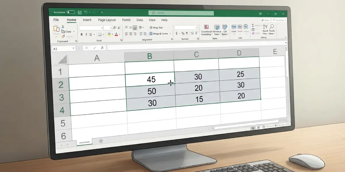
Tip: Click one cell in the data before inserting the chart. Excel then detects the whole table automatically, which prevents the common mistake of dragging a selection that misses a header or the last row.
Show Percentages Instead of Raw Numbers
A 100% stacked bar chart scales the bars to percentages, but the data labels still display the original cell values. To see actual percentages in the labels, first calculate each share in a second table (for example, the cell value divided by the row total, formatted as Percentage), and then build the chart from that table.
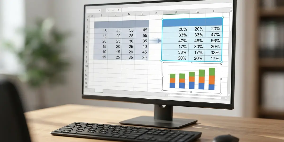
Tip: Keep the second table right beside the original one. Both stay in sync when numbers change, so the chart never needs to be rebuilt.
Common Problems and Fixes
The Bars Are Grouped the Wrong Way
Excel decides which direction to plot based on the shape of the data. Select the chart, open the Chart Design tab, and click Switch Row/Column to flip the arrangement.
The 100% Stacked Bar Option Is Missing or Greyed Out
This usually happens when no data is selected, or when a chart element is selected instead of the chart itself. Click a cell in the data range first, then open the Insert tab again.
The Category Labels Show 1, 2, 3 Instead of Names
If the first column holds numbers, such as years, Excel may treat it as a data series rather than labels. Leave the top-left header cell empty, or format the year cells as Text, and then recreate the chart.
A Series Is Missing or Shows as Zero
Numbers stored as text are ignored in the chart. Look for a small green triangle in the cell corner, click the warning icon, and choose Convert to Number.
The Chart Includes an Unwanted Total Column
If a Total column was selected with the data, each bar gets an extra segment. Right-click the chart, choose Select Data, select the Total series, and click Remove.
The Data Labels Overlap or Are Hard to Read
Click a label, open Format Data Labels, and change the font color to white or black depending on the segment color. Increasing the chart height by dragging its bottom edge also gives labels more room.
Frequently Asked Questions
What is the difference between a stacked bar chart and a 100% stacked bar chart?
A regular stacked bar chart shows actual totals, so bars have different lengths. A 100% stacked bar chart scales every bar to the same length, so only the proportions of each segment matter.
Where is the 100% stacked bar chart option in Excel?
Go to the Insert tab, click Insert Column or Bar Chart in the Charts group, and look under the 2-D Bar heading for 100% Stacked Bar.
Can a 100% stacked bar chart be created from a table that includes totals?
Yes, but the Total column should be left out of the selection. Including it adds an extra segment to every bar and distorts the percentages.
How can percentages be shown on the segments instead of the original values?
Create a helper table that divides each value by its row total and format the results as Percentage. Build the chart from that helper table, then add data labels.
Why do all the bars have the same length?
That is how the chart type works. Each bar represents 100 percent of its category, and the colored segments show how that whole is divided.
How can the order of the colored segments be changed?
Right-click the chart, choose Select Data, select a series in the list, and use the up or down arrows to move it. The segment order in every bar updates immediately.
How can the series colors be changed?
Click once on a colored segment to select the whole series, then open the Format tab and choose a new color under Shape Fill. Alternatively, use Change Colors on the Chart Design tab to apply a full palette.
Can the same steps be used on Excel for Mac?
Yes. The Insert tab, the chart gallery, and the Chart Design tab follow the same layout on Mac. Only the keyboard shortcuts differ, with Command replacing Ctrl.
How can the finished chart be moved into Word or PowerPoint?
Click the chart border, press Ctrl+C, then paste it into the other app with Ctrl+V. Use the Paste Options button to keep the chart linked to Excel or to paste it as a picture.