
Fixing the #CALC! error in Excel fast comes down to one idea: find out which kind of calculation problem the formula is hitting, then change the formula so Excel can finish the job. The error shows up when a dynamic array formula or a LAMBDA-based formula returns something Excel cannot display. The good news is that only three causes account for nearly every case, and each has a quick fix.
Key Takeaways
- #CALC! means Excel’s calculation engine hit a scenario it cannot process, most often an empty array, a nested array, or an uncalled LAMBDA.
- Evaluate Formula on the Formulas tab reveals exactly which part of the formula fails.
- For FILTER returning nothing, the if_empty argument removes the error.
- For nested arrays, make sure each step returns a single value, not a list.
- For a LAMBDA, call it with values or wrap it in a named function.
Fixing the #CALC! Error in Excel Fast: Step-by-Step
- Step 1: Click the cell that shows #CALC! and read the formula in the formula bar. Note which functions are inside it. Look for FILTER, SORT, UNIQUE, XLOOKUP, SEQUENCE, MAP, BYROW, BYCOL, REDUCE, SCAN or LAMBDA, since these are the usual suspects.
- Step 2: Open the Formulas tab, select Evaluate Formula in the Formula Auditing group, and click Evaluate repeatedly. Excel walks through the formula one calculation at a time, and the step that produces #CALC! is the part to repair.
- Step 3: Match the failing step to one of the three causes below, then apply the matching fix.
- Step 4: Press Enter to recalculate. If the result is a spill range, make sure the cells below and to the right are empty, because a blocked range produces a different error (#SPILL!).
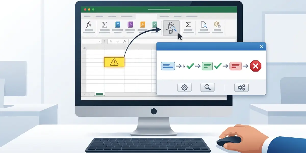
Tip: Think of Evaluate Formula as a slow-motion replay. Instead of staring at a long formula and guessing, the replay stops at the exact moment the problem happens.
Fix 1: The formula returns an empty array
This is the most common cause. A formula such as =FILTER(A2:C20, C2:C20>1000) returns #CALC! when no row meets the condition, because Excel cannot display an array with nothing in it. A sales report filtered for orders above a threshold is a typical example: in a slow month, no orders qualify and the error appears.
- Step 1: Add the third argument of FILTER, called if_empty, so the formula reads =FILTER(A2:C20, C2:C20>1000, 0).
- Step 2: To show a message instead of a number, type the message as text wrapped in quotation marks in that third argument, for example a short note saying no results were found.
- Step 3: Press Enter. The cell now shows the fallback value whenever the filter finds nothing, and the normal results as soon as matching rows exist.
The same logic applies to other functions that can return an empty array, such as SORT or UNIQUE wrapped around a FILTER. Fix the FILTER at the core and the outer functions follow.
Fix 2: The formula creates an array of arrays
Excel cannot place a list inside a single cell of another list. A formula like =BYROW(A1:C3, LAMBDA(row, row)) fails because each row returns several values instead of one. The same happens with MAP and similar functions when the LAMBDA hands back more than one value per item.
- Step 1: Use Evaluate Formula to find the inner function that returns multiple values for a single item.
- Step 2: Reduce that result to one value by wrapping it in an aggregating function. For example, =BYROW(A1:C3, LAMBDA(row, SUM(row))) returns one total per row.
- Step 3: To combine the values into one text cell, use TEXTJOIN inside the LAMBDA instead of SUM.
- Step 4: Press Enter and confirm the result spills as a simple list.
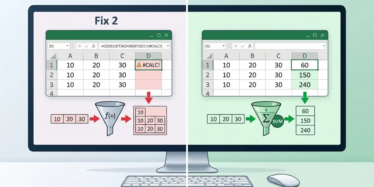
Tip: The key is to ask what each step hands back. If the answer is a list where a single value is expected, summarize it before passing it along.
Fix 3: A LAMBDA function is not being called
A LAMBDA typed straight into a cell without values behaves like a recipe with no ingredients. Entering =LAMBDA(x, x+1) alone returns #CALC! because nothing has been passed in.
- Step 1: Add the input values in parentheses right after the LAMBDA, such as =LAMBDA(x, x+1)(5).
- Step 2: For repeated use, open Formulas, then Name Manager, then New, give the LAMBDA a name, and place the LAMBDA in the Refers to box.
- Step 3: Call the named function from any cell the way a built-in function is used, for example =AddOne(5).
- Step 4: Check that the number of values passed matches the number of parameters the LAMBDA defines.
Common Problems and Fixes
The #CALC! error returns after the data changes
This usually means the formula has no safety net. A FILTER that works today can return an empty result tomorrow after a data refresh. Adding the if_empty argument makes the formula safe for every future state of the data.
The error remains after adding if_empty
Check whether a second function in the formula is also failing. Evaluate Formula often reveals two problems stacked together, such as an empty FILTER followed by a BYROW that returns lists.
The fix works, but a #SPILL! error appears
The formula now calculates, but something is blocking the spill range. Clear the cells below and to the right of the formula, or move the formula to an open area of the sheet.
The LAMBDA works in one workbook but not another
Named LAMBDA functions are stored per workbook. Recreate the name in Name Manager in the new workbook, or copy the sheet that contains the named function.
The formula opens fine on one computer and shows #CALC! on another
Older Excel versions without dynamic array support cannot calculate these functions. Confirm that the second computer runs Microsoft 365 or a recent Excel version that includes FILTER, MAP and LAMBDA.
Frequently Asked Questions
What does the #CALC! error mean in Excel?
It means Excel’s calculation engine ran into a scenario it cannot process. The most common triggers are an empty array, an array nested inside another array, and a LAMBDA that has not been called with values.
Why does FILTER return #CALC! in Excel?
FILTER returns #CALC! when no rows match the condition, because the result is an empty array. Adding the if_empty argument tells Excel what to show instead.
How do I stop #CALC! from appearing when a FILTER finds nothing?
Fill in the third argument of FILTER with a fallback, such as 0 or a text message in quotation marks. The cell then displays that fallback whenever no data matches.
Can IFERROR hide the #CALC! error?
Yes, wrapping the formula in IFERROR replaces the error with a value of choice. The if_empty argument is cleaner for FILTER, since IFERROR can also hide unrelated problems that deserve attention.
What is a nested array, and why does it cause #CALC!?
A nested array is a list placed inside a single cell of another list. Excel cannot display that structure, so the formula must return one value per item instead.
Why does my LAMBDA formula show #CALC!?
The LAMBDA was probably entered without being called. Add the input values in parentheses after the LAMBDA, or save it in Name Manager and call it by name.
How can I find which part of a formula causes #CALC!?
Select the cell, open the Formulas tab, and use Evaluate Formula. Each click on Evaluate runs one step, and the step that produces the error points to the cause.
Is #CALC! the same as #SPILL!?
No. #SPILL! means the results are ready but something blocks the cells where they should appear. #CALC! means Excel could not complete the calculation itself.
Does the #CALC! error appear in older versions of Excel?
The error belongs to the dynamic array and LAMBDA features found in Microsoft 365 and recent Excel versions. Older versions that lack those functions show a different error, such as #NAME?, instead.